06_1970년대 보스톤 지역의 주택 가격 예측.ipynb

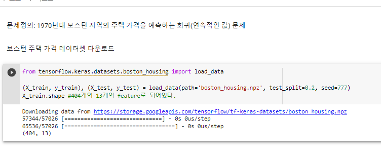
^ 보스턴 주택 가격 데이터셋 다운로드

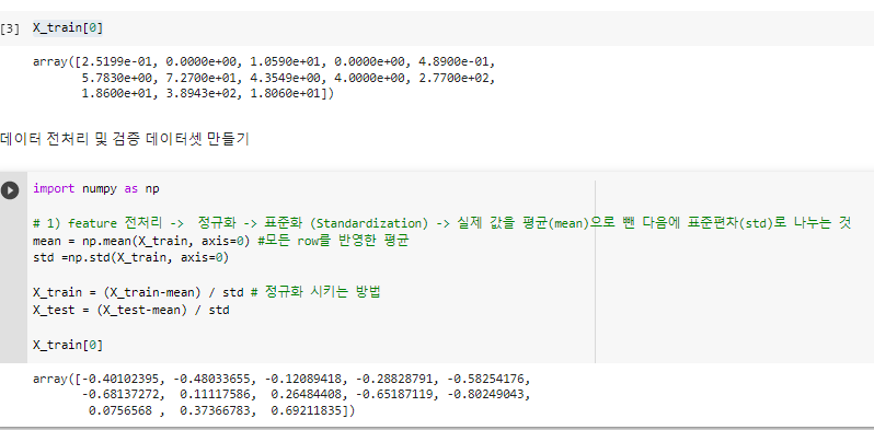
^ 데이터 전처리 통해 평균값들을 구할 수 있다.

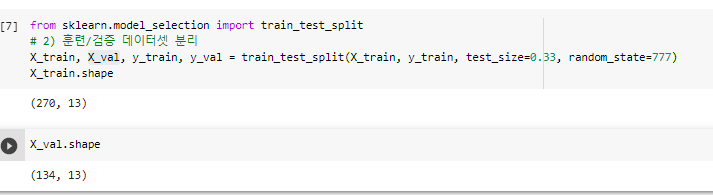
^ "270개로, 134개로 검증을 해보겠다"

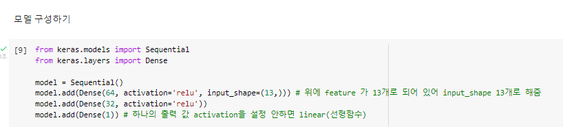
^ 모델 구성하기

^ 모델 설정하기

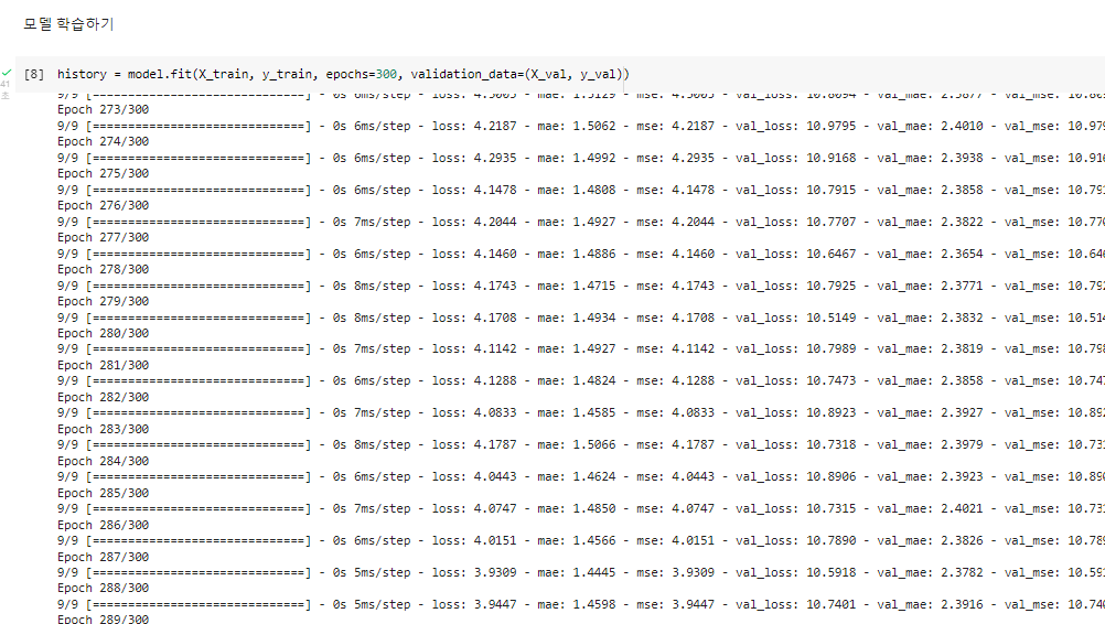
^ 모델 학습하기

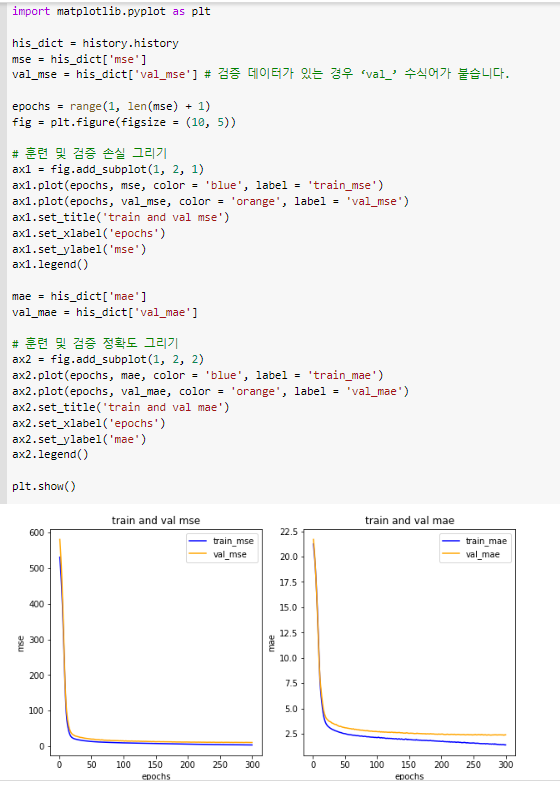
import matplotlib.pyplot as plt

his_dict = history.history
mse = his_dict['mse']
val_mse = his_dict['val_mse'] # 검증 데이터가 있는 경우 ‘val_’ 수식어가 붙습니다.

epochs = range(1, len(mse) + 1)
fig = plt.figure(figsize = (10, 5))

# 훈련 및 검증 손실 그리기
ax1 = fig.add_subplot(1, 2, 1)
ax1.plot(epochs, mse, color = 'blue', label = 'train_mse')
ax1.plot(epochs, val_mse, color = 'orange', label = 'val_mse')
ax1.set_title('train and val mse')
ax1.set_xlabel('epochs')
ax1.set_ylabel('mse')
ax1.legend()

mae = his_dict['mae']
val_mae = his_dict['val_mae']

# 훈련 및 검증 정확도 그리기
ax2 = fig.add_subplot(1, 2, 2)
ax2.plot(epochs, mae, color = 'blue', label = 'train_mae')
ax2.plot(epochs, val_mae, color = 'orange', label = 'val_mae')
ax2.set_title('train and val mae')
ax2.set_xlabel('epochs')
ax2.set_ylabel('mae')
ax2.legend()

plt.show()

^ 그리기

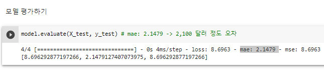
^ 모델 평가하기

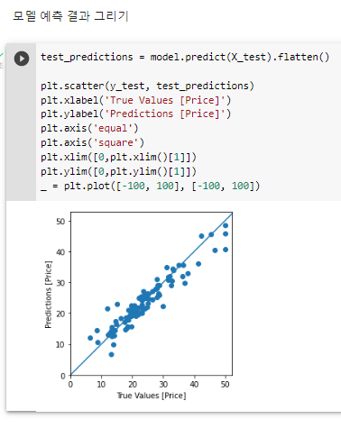
test_predictions = model.predict(X_test).flatten()

plt.scatter(y_test, test_predictions)
plt.xlabel('True Values [Price]')
plt.ylabel('Predictions [Price]')
plt.axis('equal')
plt.axis('square')
plt.xlim([0,plt.xlim()[1]])
plt.ylim([0,plt.ylim()[1]])
_ = plt.plot([-100, 100], [-100, 100])

# 이 모델이 집값을 조금 더 싸게 예측하는 경우가 있다.

^ 모델 예측 결과 그리기

from tensorflow.keras.datasets.boston_housing import load_data
from tensorflow.keras.models import Sequential
from tensorflow.keras.layers import Dense

import numpy as np
from sklearn.model_selection import KFold

(x_train, y_train), (x_test, y_test) = load_data(path='boston_housing.npz',
                                                 test_split=0.2,
                                                 seed=777)

# 데이터 표준화
mean = np.mean(x_train, axis = 0)
std = np.std(x_train, axis = 0)
# 여기까진 전부 동일합니다.
x_train = (x_train - mean) / std
x_test = (x_test - mean) / std

#----------------------------------------
# K-Fold를 진행해봅니다.
k = 3

# 주어진 데이터셋을 k만큼 등분합니다.
# 여기서는 3이므로 훈련 데이터셋(404개)를 3등분하여
# 1개는 검증셋으로, 나머지 2개는 훈련셋으로 활용합니다.
kfold = KFold(n_splits=k)

# 재사용을 위해 모델을 반환하는 함수를 정의합니다.

def get_model():
    model = Sequential()
    model.add(Dense(64, activation = 'relu', input_shape = (13, )))
    model.add(Dense(32, activation = 'relu')) 
    model.add(Dense(1))   

    model.compile(optimizer = 'adam', loss = 'mse', metrics = ['mae'])
    
    return model

mae_list = [] # 테스트셋을 평가한 후 결과 mae를 담을 리스트를 선언합니다.

# k번 진행합니다.
for train_index, val_index in kfold.split(x_train):
    # 해당 인덱스는 무작위로 생성됩니다.
    # 무작위로 생성해주는 것은 과대적합을 피할 수 있는 좋은 방법입니다.
    x_train_fold, x_val_fold = x_train[train_index], x_train[val_index]
    y_train_fold, y_val_fold = y_train[train_index], y_train[val_index]
    
    # 모델을 불러옵니다.
    model = get_model()
    
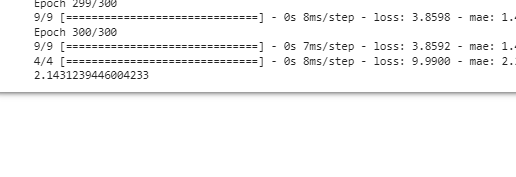
    model.fit(x_train_fold, y_train_fold, epochs = 300, validation_data = (x_val_fold, y_val_fold))
    
    _, test_mae = model.evaluate(x_test, y_test)
    mae_list.append(test_mae)

print(np.mean(mae_list)) 

^ Kfold