(2018)VoxelMorph: A Learning Framework for Deformable Medical Image Registration
Paper Review
0. Abstract
전통적인 image registration은 paired images간의 objective function을 최적화하는 방식이며 시간이 많이 소요된다.
반대로 본 논문의 접근 방법은 최근에 제안이 된 학습 기반의 방법이며 registration을 하나의 함수로 보고 input image를 넣으면 align이 된 image가 나오게 된다.
본 논문에서는 두 가지의 접근 법을 제안한다. 첫 번째로 unsupervised learning으로 image간의 matching objective function을 최적화한다. 두 번째로 auxiliary segmentation map을 학습에 활용한다.
제안 된 unsupervised model은 SOTA 방법들과 비교했을 때 경쟁력 있는 결과를 보여주며 연산 속도는 매우 빠르다. 또한 auxiliary data를 사용했을 때 registration 성능이 올라갔다.
1. Introduction
Image registration에서 deformable registration은 가장 대표적인 방법이다. 하지만 연산 시간이 매우 오래 걸린다는 단점이 있다.
본 논문에서는 unsupervised learning으로 paired images의 volume pair만을 사용해 학습을 했고 anatomical segmentation map을 학습에 사용해 성능을 높였다.
테스트 시 여러 study의 다양한 연령대, 정상인과 뇌 질환 환자가 섞인 3500장의 scan을 사용했다. 제안 된 model은 CPU를 사용 시 몇 분 이내, GPU를 사용 시 몇 초 이내에 연산이 끝나지만 현재 SOTA인 방법은 수 십분에서 2시간 가량의 시간이 소요된다.
2. Background
일반적으로 deformable registration은 global alignment를 찾고 deformable transformation을 구하는 두 step으로 나눠진다.
본 논문에서는 두 번째 step에서 모든 voxel에 대한 dense, nonlinear correspondence를 계산하는 것에 집중한다.
전통적인 방식은 volume pair를 최적화하는 방식으로 많은 시간이 소요된다. 반대로 본 논문에서는 data로 부터 deformable field를 생성하는 parameterized function을 구할 수 있다고 가정한다. 즉, pair-specific optimization이 아니라 global optimization인 것이다.
3. Related Work
Non-learning-based 방식으로는 elastic type model, statistical parametric mapping, b-splines, discrete methods, demons와 같은 방법들이 있다.
Diffeomorphic transforms은 뛰어난 성능을 보여줬는데 LDDMM(Large Diffeomorphic Distance Metric Mapping), DARTEL, diffeomorphic demons, SyN(Symmetric normalization)과 같은 방법들이 있다.
모든 non-learning-based 방식들은 energy function을 optimize하는 접근 방법이며 연산 시간이 매우 오래 걸린다는 단점이 있다.
최근에 제안 된 image registration을 위한 neural networks들은 ground truth warp fields에 의존한다는 단점이 있다. 이는 deformation을 수행해야 얻을 수 있기 때문에 수고가 든다.
반대로 본 논문에서 VoxelMorph는 unsupervised learning이며 segmentation map과 같은 auxiliary information을 사용해 성능을 더욱 높였다.
4. Method

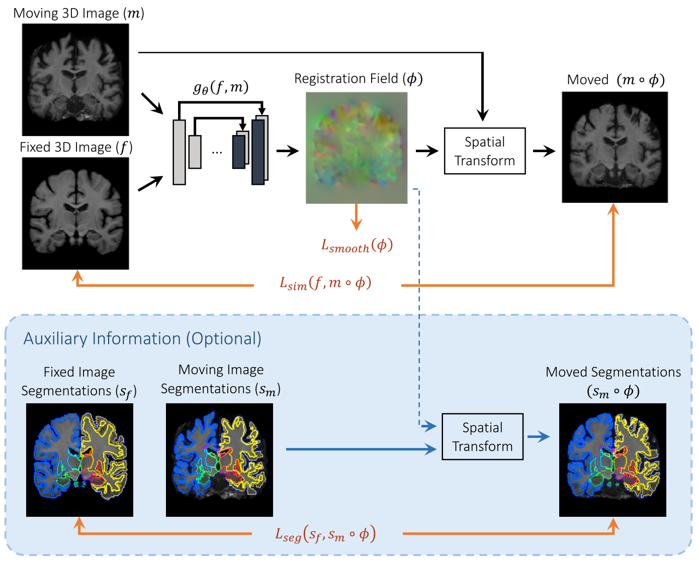
먼저 사전에 affine alignment를 수행하고 그 후에 misalignment는 nonlinear라고 가정하고 들어간다. 위 그림에서 함수 는 CNN이고 는 network의 parameters이다.
Fixed image 와 moving image 이 입력되면 parameters 를 통해 를 계산한다.
그리고 와 의 similarity를 계산한다.
Stochastic gradient descent 방식으로 optimal parameters인 를 loss function을 minimizing 하면서 업데이트 해 나가게 된다. 본 논문에서는 두 가지 loss를 제안하였는데 similarity와 field smoothness loss이다.
A. VoxelMorph CNN Architecture
.png)
는 encoder, decoder, skip connections로 구성된 UNet기반의 CNN이다.
하나의 input이 있으며 과 를 concatenating한 size의 image가 입력으로 들어간다. Input size는 고정이 아니며 변경이 가능하다.
B. Spatial Transformation Function
제안 된 방법은 와 간의 차이를 최소화하는 최적의 parameter를 학습한다.
그리고 학습이 완료되면 의 voxel 마다 를 계산한다. Image의 value는 integer location에서 정의 되기 때문에 linear interpolation을 이용해 eight neighboring voxel을 다음과 같이 계산한다.p
는 의 이웃 voxel이며 는 dimension을 나타낸다.
C. Loss Functions
1) Unsupervised Loss Function
Unsupervised loss는 appearance의 차이를 고려하는 similarity loss 과 의 local spatial variations를 고려하는 smoothness loss 로 구성된다. 는 regularization parameter이다.
Similarity loss는 두 가지를 실험에 사용하였다. 첫 번째는 와 이 비슷한 intensity distribution과 local contrast를 가질 때 적용이 가능한 mean squared voxelwise difference이다.
두 번째는 intensity의 variation에 좀 더 robust한 local cross-correlation이다.
와 는 local mean intensity를 나타내며 다음과 같이 계산된다.
Local cross-correlation 전체 식은 다음과 같다.
을 최소화 하는 것은 를 에 근접하게 할 수 있으나 realistic하지 않은 non-smooth 를 생성할 수 있다. 이를 해결하기 위해 diffusion regularizer를 이용해 smoothness loss를 적용하였다.
2) Auxiliary Data Loss Function
Anatomical segmentation maps는 학습에만 사용이 되며 전문가나 automated algorithm을 사용함으로 annotation이 가능하다.
만약 registration field 가 정확한 anatomical correspondence를 가진다면 와 의 anatomical structure 또한 overlap이 잘 되어야 한다.
본 논문에서는 volume overlap을 Dice score로 정량화 하였다. 는 structure의 class이다.
위 두 가지 loss를 조합해서 total loss를 구성한다. 는 regularization parameter이다.
5. Experiments
A. Experimental Setup
1) Dataset
다양한 연구, 다양한 장소에서 얻은 3731 volume의 T1-weighted brain MRI scan을 사용하였다. 모든 scan은 의 1mm isotropic voxel로 구성되어 있다.
앞서 FreeSurfer로 기본적인 affine spatial normalization과 brain extraction을 수행하였다.
모든 데이터는 FreeSurfer를 이용해 anatomical segmentation maps를 얻었다. 그리고 visual inspection으로 segmentation map의 오류를 수정하였다.
Train 3231, validation 250, test 250 volume을 사용하였다.
2) Evaluation Metrics
Anatomical structure의 overlap을 평가하기 위해 Dice score를 사용하였다.
Deformation fields의 regularity를 평가하기 위해 Jacobian determinant를 사용하였다.
인 non-background voxels를 count한다.
3) Baseline Methods
비교 methods로 ANTs SyN과 NiftyReg를 사용하였다.
본 논문의 VoxelMorph의 implementation은 Keras를 사용하였고 optimizer는 ADAM, learning rate는 이다.
B. Atlas-based Registration
.png)
VoxelMorph는 atlas-based registration이다. 위 그림은 moving image , atlas인 fixed image , deformation fields 를 나타내고 있다.
.png)
Dice score를 비교한 결과 다른 method와 견줄만한 성능을 보여줬을 뿐만 아니라 속도는 매우 빠르다. Jacobian determinant는 모두 1%이내의 성능을 보여줬다.
.png)
위 그래프는 training set의 size에 따른 Dice score의 변화를 보여준다. 약간의 차이가 있으나 dataset의 크기에 따른 Dice score의 변화는 크지 않는 것으로 보인다.
.png)
일 때, 가장 Dice score가 좋고 irregular deformation fields를 피할 수 있었다.
6. Discussion and Conclusion
VoxelMorph는 수 십분에서 수 시간이 걸리는 연산 시간을 수 분에서 몇 초 이내로 줄였을 뿐만 아니라 Dice score 성능에서도 ANTs, NiftyReg와 견줄만한 성능을 보여줬다.
또한 100 volume의 dataset만으로도 좋은 성능을 보여주기 때문에 많은 양의 dataset이 필요하지 않다.
VoxelMorph는 learning-based model이다. 그리고 특정한 image의 type이나 anatomy에 제한 받지 않는다. 이는 cardiac MR scans나 lung CT images에도 유용하게 사용될 수 있을 것으로 보인다. 또한 mutual information과 같은 적절한 loss를 사용한다면 multi-modal registration에도 사용이 가능하다.
VoxelMorph는 medical image의 analysis와 processing pipelines에 상당한 속도의 향상을 주었을 뿐만 아니라 learning-based registration에 새로운 방향을 제시하였다.
