Trust Region PO vs Proximal PO
PPO는 이전 TRPO 알고리즘을 조금 더 실용적으로 발전시킨 논문
Policy gradient 계열의 알고리즘으로, 성능이 우수하면서도 구현이 간단하여 performance와 complexity 간의 밸런스가 잘 잡힌 알고리즘으로 알려짐
PPO와 TRPO는 주어진 데이터로 현재 policy를 최대한 큰 step만큼 빠르게 향상시키면서, 너무 발산할 정도로 큰 step으로 업데이트하는 것은 억제하고자 하는 동일한 motivation을 가짐
TRPO : maximize θ E ^ t [ π θ ( a t ∣ s t ) π old ( a t ∣ s t ) A ^ t − β K L [ π old ( ⋅ ∣ s t ) ∣ ∣ π θ ( ⋅ ∣ s t ) ] ] PPO : maximize θ E ^ t [ min ( π θ ( a t ∣ s t ) π old ( a t ∣ s t ) A ^ t , clip ( π θ ( a t ∣ s t ) π old ( a t ∣ s t ) , 1 − ϵ , 1 + ϵ ) A ^ t ) ] \text{TRPO}:\;\text{maximize}_\theta\;\hat{\mathbb{E}}_t[\frac{\pi_\theta(a_t|s_t)}{\pi_\text{old}(a_t|s_t)}\hat{A}_t-\beta KL[\pi_\text{old}(\cdot|s_t)\,||\,\pi_\theta(\cdot|s_t)]] \\ \;\;\,\text{PPO}:\;\text{maximize}_\theta\;\hat{\mathbb{E}}_t[\min(\frac{\pi_\theta(a_t|s_t)}{\pi_\text{old}(a_t|s_t)}\hat{A}_t,\;\text{clip}(\frac{\pi_\theta(a_t|s_t)}{\pi_\text{old}(a_t|s_t)},1-\epsilon,1+\epsilon)\hat{A}_t)] TRPO : maximize θ E ^ t [ π old ( a t ∣ s t ) π θ ( a t ∣ s t ) A ^ t − β K L [ π old ( ⋅ ∣ s t ) ∣ ∣ π θ ( ⋅ ∣ s t ) ] ] PPO : maximize θ E ^ t [ min ( π old ( a t ∣ s t ) π θ ( a t ∣ s t ) A ^ t , clip ( π old ( a t ∣ s t ) π θ ( a t ∣ s t ) , 1 − ϵ , 1 + ϵ ) A ^ t ) ]
TRPO에서는 objective term π θ ( a ∣ s ) π old ( a ∣ s ) A ^ t \frac{\pi_\theta(a|s)}{\pi_\text{old}(a|s)}\hat{A}_t π old ( a ∣ s ) π θ ( a ∣ s ) A ^ t K L [ π old ∣ ∣ π θ ] KL[\pi_\text{old}||\pi_\theta] K L [ π old ∣ ∣ π θ ]
즉 목적식을 통해 policy의 improvement step을 최대한 크게 가져가면서, 동시에 penalty term에서 old policy와 new policy 간의 차이가 너무 커지지 않도록 KL divergence를 통해 제한하는 역할까지
PPO에서는 objective term π θ ( a ∣ s ) π old ( a ∣ s ) A ^ t \frac{\pi_\theta(a|s)}{\pi_\text{old}(a|s)}\hat{A}_t π old ( a ∣ s ) π θ ( a ∣ s ) A ^ t
이를 통해 second-order method가 아닌 first-order method로 계산이 가능해져 구현 상의 실용성을 얻게 됨
PPO의 메커니즘
Surrogate Objective
Policy gradient 알고리즘은 목적 함수 J ( π θ ) J(\pi_\theta) J ( π θ ) ∇ J \nabla J ∇ J π θ \pi_\theta π θ J ( π θ ) = E s ∼ ρ π θ , a ∼ π θ [ A π θ ] = ∑ s ρ π θ ( s ) ∑ a π θ ( a ∣ s ) A π θ ( s , a ) J(\pi_\theta)=\mathbb{E}_{s\sim\rho_{\pi_\theta},a\sim\pi_\theta}[A_{\pi_\theta}]=\sum_s\rho_{\pi_\theta}(s)\sum_a\pi_\theta(a|s)A_{\pi_\theta}(s,a) J ( π θ ) = E s ∼ ρ π θ , a ∼ π θ [ A π θ ] = s ∑ ρ π θ ( s ) a ∑ π θ ( a ∣ s ) A π θ ( s , a )
목적함수를 어떻게 정의했는지에 따라 policy gradient는 다양하게 표현할 수 있으며, advantage A π θ A_{\pi_\theta} A π θ
ρ π θ ( s ) = P ( s 0 = s ) + γ P ( s 1 = s ) + γ 2 P ( s 2 = s ) + ⋯ \rho_{\pi_\theta}(s)=P(s_0=s)+\gamma P(s_1=s)+\gamma^2 P(s_2=s)+\cdots ρ π θ ( s ) = P ( s 0 = s ) + γ P ( s 1 = s ) + γ 2 P ( s 2 = s ) + ⋯ s s s
여기서 π old → π θ \pi_\text{old}\rightarrow\pi_\theta π old → π θ ρ π θ ( s ) \rho_{\pi_\theta}(s) ρ π θ ( s ) ρ π old ( s ) \rho_{\pi_\text{old}}(s) ρ π old ( s ) L ( π θ ) L(\pi_\theta) L ( π θ ) J ( π θ ) = ∑ s ρ π θ ( s ) ∑ a π θ ( a ∣ s ) A π θ ( s , a ) L ( π θ ) = ∑ s ρ π old ( s ) ∑ a π θ ( a ∣ s ) A π θ ( s , a ) J(\pi_\theta)=\sum_s\rho_{\pi_\theta}(s)\sum_a\pi_\theta(a|s)A_{\pi_\theta}(s,a) \\ L(\pi_\theta)=\sum_s\rho_{\pi_\text{old}}(s)\sum_a\pi_\theta(a|s)A_{\pi_\theta}(s,a) J ( π θ ) = s ∑ ρ π θ ( s ) a ∑ π θ ( a ∣ s ) A π θ ( s , a ) L ( π θ ) = s ∑ ρ π old ( s ) a ∑ π θ ( a ∣ s ) A π θ ( s , a )
따라서, policy가 충분히 작은 만큼만 변화했을 때는 J ( π θ ) J(\pi_\theta) J ( π θ ) L ( π θ ) L(\pi_\theta) L ( π θ )
이 때문에 policy update에 대한 constraint가 추후 penalty term으로 추가됨
Importance Sampling
[Importance Sampling] f ( x ) f(x) f ( x ) p ( x ) p(x) p ( x ) E x ∼ p [ f ( x ) ] = ∫ f ( x ) p ( x ) d x \mathbb{E}_{x\sim p}[f(x)]=\int f(x)p(x)dx E x ∼ p [ f ( x ) ] = ∫ f ( x ) p ( x ) d x x ( n ) x^{(n)} x ( n ) p ( x ) p(x) p ( x ) q ( x ) q(x) q ( x ) E x ∼ p [ f ( x ) ] \mathbb{E}_{x\sim p}[f(x)] E x ∼ p [ f ( x ) ]
E x ∼ p [ f ( x ) ] ≃ 1 N ∑ n = 1 N f ( x ( n ) ) ⏟ Monte Carlo ≃ 1 N ∑ n = 1 N p ( x ) q ( x ) f ( x ( n ) ) ⏟ Importance Sampling \mathbb{E}_{x\sim p}[f(x)] \simeq \underset{\text{Monte Carlo}}{\underbrace{\frac{1}{N}\sum^N_{n=1}f(x^{(n)})}} \simeq\underset{\text{Importance Sampling}}{\underbrace{\frac{1}{N}\sum^N_{n=1}\frac{p(x)}{q(x)}f(x^{(n)})}} E x ∼ p [ f ( x ) ] ≃ Monte Carlo N 1 n = 1 ∑ N f ( x ( n ) ) ≃ Importance Sampling N 1 n = 1 ∑ N q ( x ) p ( x ) f ( x ( n ) ) x ∼ p x\sim p x ∼ p
Sample 기반 추정을 위해 surrogate objective를 expectation으로 표현하고, importance sampling을 활용해 식을 변형하면 아래와 같이 나타낼 수 있음L ( π θ ) = E s ∼ ρ π old , a ∼ π θ [ A π θ ( s , a ) ] = E s ∼ ρ π old , a ∼ π old [ π θ ( a ∣ s ) π old ( a ∣ s ) A π θ ( s , a ) ] L(\pi_\theta) =\mathbb{E}_{s\sim\rho_{\pi_\text{old}},a\sim\pi_\theta}[A_{\pi_\theta}(s,a)] =\mathbb{E}_{s\sim\rho_{\pi_\text{old}},a\sim\pi_\text{old}}[\frac{\pi_\theta(a|s)}{\pi_\text{old}(a|s)}A_{\pi_\theta}(s,a)] L ( π θ ) = E s ∼ ρ π old , a ∼ π θ [ A π θ ( s , a ) ] = E s ∼ ρ π old , a ∼ π old [ π old ( a ∣ s ) π θ ( a ∣ s ) A π θ ( s , a ) ]
Importance sampling을 통해 기존 policy π old \pi_\text{old} π old π θ \pi_\theta π θ
즉, 새로 업데이트 된 policy를 평가할 때마다 새로운 sample을 생성할 필요 없이 old policy로부터 생성된 sample을 재사용할 수 있다는 뜻
E ^ t \hat{\mathbb{E}}_t E ^ t L ( θ ) = E ^ t [ π θ ( a t ∣ s t ) π old ( a t ∣ s t ) A ^ t ] L(\theta)=\hat{\mathbb{E}}_t[\frac{\pi_\theta(a_t|s_t)}{\pi_\text{old}(a_t|s_t)}\hat{A}_t] L ( θ ) = E ^ t [ π old ( a t ∣ s t ) π θ ( a t ∣ s t ) A ^ t ]
이로 인해 PPO는 한 번의 episode에서 획득한 sample들을 여러 번 재사용해 policy 업데이트를 할 수 있음
Clipping
Policy의 과도한 업데이트를 막기 위해 PPO는 clipping과 adaptive KL penalty의 두 방식을 제안했으나, 일반적으로 clipping 방식이 널리 알려져 있음
Surrogate objective에서 r t ( θ ) = π θ ( a t ∣ s t ) π old ( a t ∣ s t ) r_t(\theta)=\frac{\pi_\theta(a_t|s_t)}{\pi_\text{old}(a_t|s_t)} r t ( θ ) = π old ( a t ∣ s t ) π θ ( a t ∣ s t )
때문에 policy가 업데이트 되지 않아 π θ = π old \pi_\theta=\pi_\text{old} π θ = π old r t ( θ ) = 1 r_t(\theta)=1 r t ( θ ) = 1
Clipping은 이 r t ( θ ) r_t(\theta) r t ( θ ) [ 1 − ϵ , 1 + ϵ ] [1-\epsilon,1+\epsilon] [ 1 − ϵ , 1 + ϵ ]
L CLIP ( θ ) = min ( r t ( θ ) A ^ t , clip ( r t ( θ ) , 1 − ϵ , 1 + ϵ ) ) L^\text{CLIP}(\theta)=\min(r_t(\theta)\hat{A}_t,\;\text{clip}(r_t(\theta),1-\epsilon,1+\epsilon)) L CLIP ( θ ) = min ( r t ( θ ) A ^ t , clip ( r t ( θ ) , 1 − ϵ , 1 + ϵ ) )
Clipping은 최종적으로는 위 수식처럼 r t ( θ ) A ^ t r_t(\theta)\hat{A}_t r t ( θ ) A ^ t clip ( r t ( θ ) , 1 − ϵ , 1 + ϵ ) \text{clip}(r_t(\theta),1-\epsilon,1+\epsilon) clip ( r t ( θ ) , 1 − ϵ , 1 + ϵ )
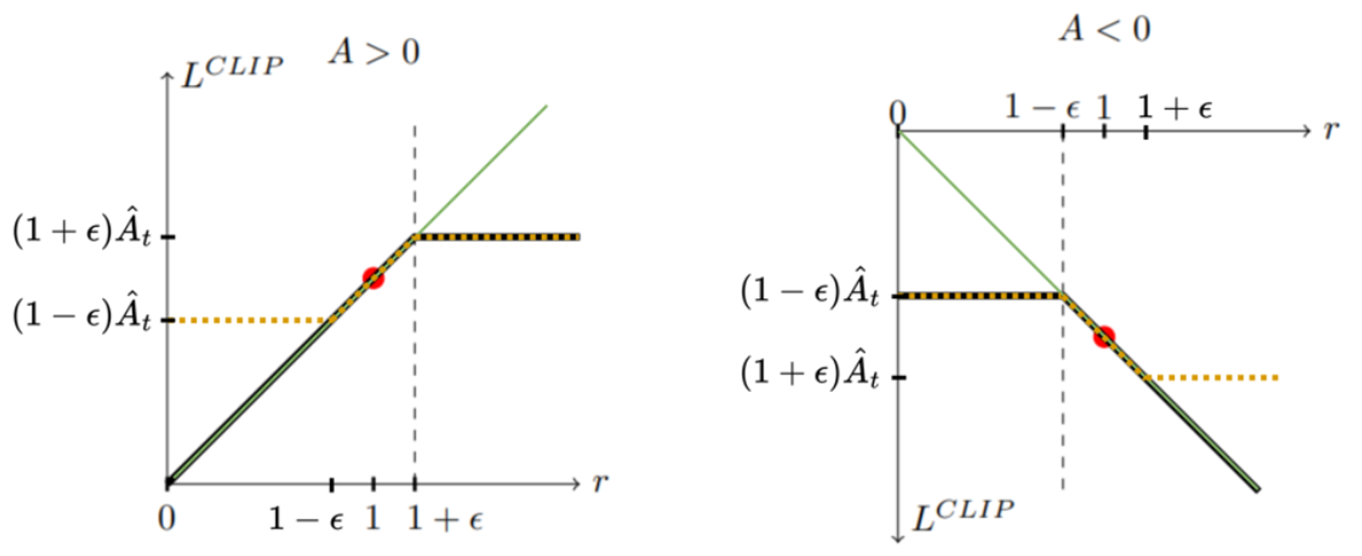
결과적으로 advantage가 양수일 때는 1 + ϵ 1+\epsilon 1 + ϵ 1 − ϵ 1-\epsilon 1 − ϵ
L CLIP L^\text{CLIP} L CLIP
A > 0 A>0 A > 0 r r r L CLIP L^\text{CLIP} L CLIP A < 0 A<0 A < 0 r r r L CLIP L^\text{CLIP} L CLIP 여기서 PPO는 A > 0 A>0 A > 0 1 + ϵ 1+\epsilon 1 + ϵ r r r A < 0 A<0 A < 0 1 − ϵ 1-\epsilon 1 − ϵ r r r L CLIP L^\text{CLIP} L CLIP
Generalized Advantage Estimation (GAE)
Trajectory로부터 추정된 기존의 advantage는 high variance error를 가지고 있음Advantage function : A ^ t = − V ( s t ) + r t + γ r t + 1 + ⋯ + γ T − t + 1 r T − 1 + γ T − t V ( s T ) (Truncated) GAE : A ^ t = δ t + ( γ λ ) δ t + 1 + ⋯ + ( γ λ ) T − t + 1 δ T − 1 where δ t = r t + γ V ( s t + 1 ) − V ( s t ) \text{Advantage function}: \quad\hat{A}_t=-V(s_t)+r_t+\gamma r_{t+1}+\cdots+\gamma^{T-t+1}r_{T-1}+\gamma^{T-t}V(s_T) \\ \text{(Truncated) GAE}: \quad\hat{A}_t=\delta_t+(\gamma\lambda)\delta_{t+1}+\cdots+(\gamma\lambda)^{T-t+1}\delta_{T-1} \\ \quad\text{where}\quad\delta_t=r_t+\gamma V(s_{t+1})-V(s_t) Advantage function : A ^ t = − V ( s t ) + r t + γ r t + 1 + ⋯ + γ T − t + 1 r T − 1 + γ T − t V ( s T ) (Truncated) GAE : A ^ t = δ t + ( γ λ ) δ t + 1 + ⋯ + ( γ λ ) T − t + 1 δ T − 1 where δ t = r t + γ V ( s t + 1 ) − V ( s t )
PPO에서는 기존의 advantage variance를 낮추기 위해 truncated GAE를 사용
GAE는 파라미터 λ \lambda λ λ = 0 \lambda=0 λ = 0 λ = 1 \lambda=1 λ = 1
PPO 알고리즘
[Pseudo code of PPO algorithm]
for iteration=1, 2, ..., N do
    for actor=1, 2, ..., N do
        Run policy π_{θ_old} in environment for T timesteps
        Compute advantage estimates Â_1, ..., Â_t
    end for
    Optimize surrogate L w.r.t. θ, with K epochs and minibatch size M ≤ NT
    θ_old ← θ
end for
PPO는 environment와의 상호 작용 시 한 번의 step만 진행해야할 필요는 없으며, 고정된 길이의 trajectory (또는 episode) 단위로 상호작용할 수 있음
또한 여러 actor를 병렬 수행해 sample을 획득할 수 있음
따라서, 해당 과적으로는 N N N T T T
결과적으로 N T NT N T
PPO는 importance sampling으로 surrogate objective를 최적화하기 위한 파라미터 업데이트를 K K K