Ch.1 Filtering

Types of Image Transformation

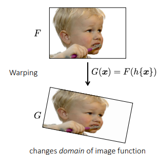
What is an image?

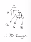
(컬러) 이미지는 3D텐서: weight, height, color

R:8bit / G:8bit / B:8bit (→24bit)
min: 0 (black) / max: 255 (white)

(흑백; grayscale) 이미지는 2D 함수

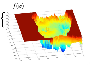
• 색깔 intensity 정규화 (0~255 → 0~1)

What types of image transformations can we do?

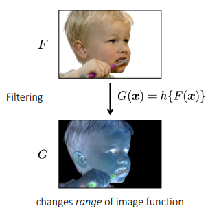
What types of image filtering can we do?

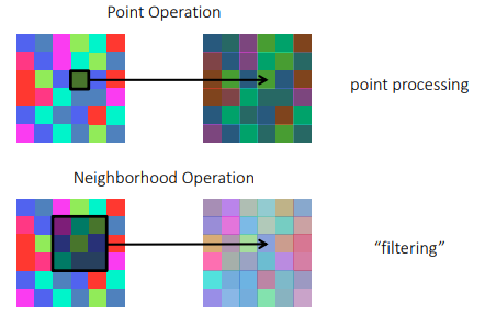
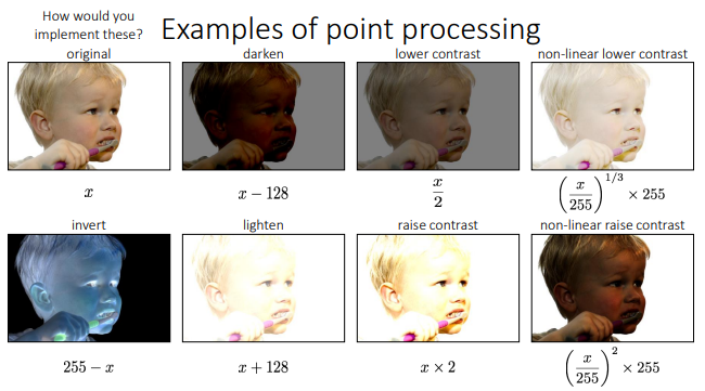
Point Image Processing

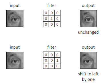
Linear Shift-Invariant Image Filtering

Replace each pixel by a linear combination of its neighbors (and possibly itself)

linear combination (선형결합)
여러개의 벡터에 스칼라 곱을 한 뒤, 그 결과들을 더하는 것
결합 방식은 필터의 커널에 의해 결정됨
동일한 커널이 모든 픽셀위치로 이동 → 모든 픽셀이 이웃 픽셀과 동일한 선형 결합 사용

Box Filter

2D rect filter / square mean filter 라고도 불림

blurring effect box filter

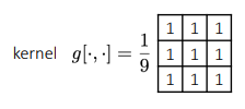
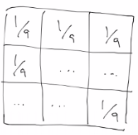
= local 평균값으로 각 픽셀 교체

$k * k$ 커널일때,
$k//2 =$ 중심 픽셀로부터 이웃 픽셀까지 거리
ex) $3*3$ 커널일때, $k//2 = 1$, 즉 주변 1개씩

Convolution

커널을 뒤집어서 선형결합 진행

• 커널이 대칭이면, filtering = convolution

Convolution for 1D continuous signals

• $(f*g)(x)$ : filtered signal
• $f(y)$ : filter
• $g(x-y)$ : input signal
  • flip 확인

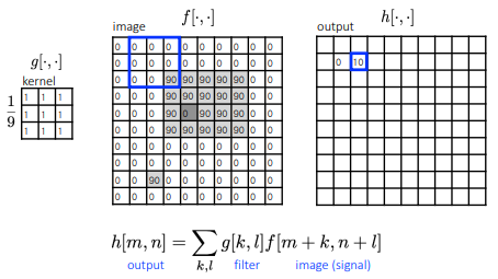
Convolution for 2D discrete signals

• $(f*g)(x,y)$ : filtered image
• $f(i,j)$ : filter
• $I(x-i, y-j)$ : input image
  • flip 확인

Convolution vs Correlation

Definition of discrete 2D Convolution:

$(f*g)(x,y) = \sum_{i,j = -\infty}^{\infty} f(i,j) I(x-i, y-j)$

Definition of discrete 2D Convolution:

$(f*g)(x,y) = \sum_{i,j = -\infty}^{\infty} f(i,j) I(x+i, y+j)$

• 차이점은 커널의 flip 여부
• 대부분 커널은 대칭이라 별 차이 없음
• convolution: 신호처리에 많이 쓰임 (ex. filtering, blurring, edge detection 등)
• correlation: 두 신호 or 함수의 유사도 측정에 많이 쓰임 (ex. template matching)

Seperable Filters

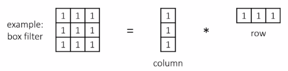
원래 이미지 M x M, 필터 커널 N x N 일때,

기존 시간 복잡도: $(M * M) * (N * N) = O(M^2N^2)$

Seperable Filter 시간 복잡도: $2 * {(M * M) * N} = O(2M^2N)$

▶ 훨씬 빠름

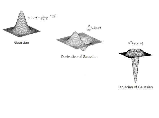
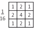
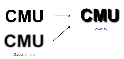
Gaussian Filter

Soft Shadow Effect

Other filters

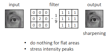
• sharpening 너무 많이 하면 노이즈 ↑

Image Gradients

What are image edges?

very sharp discontinuities in intensity

• 미분 = 기울기

$\nabla = \sqrt {{\nabla x}^2 + {\nabla y}^2}$
→ 총 기울기 = |(x기울기) + (y기울기)|

Detecting edges

미분값은 불연속성이 있는 부분(=edge)에서 큼

미분 값을 구하기 위해 finite differences 활용

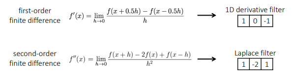
Finite Differences

1. 우극한

2. 좌극한

3. 중앙차분

4. For discrete signals

극한이 아니라, h=2로 둠

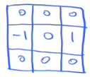
1D derivative filter

• if convolution:

The Sobel Filter

위 필터는 미분만 수행 → noise↑

horizontal sobel filter

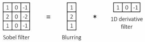
가우시안 필터 (blur) * 1차원 미분 필터 (horizontal)

• horizontal 필터 → vertical edge 찾아냄

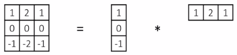
vertical sobel filter

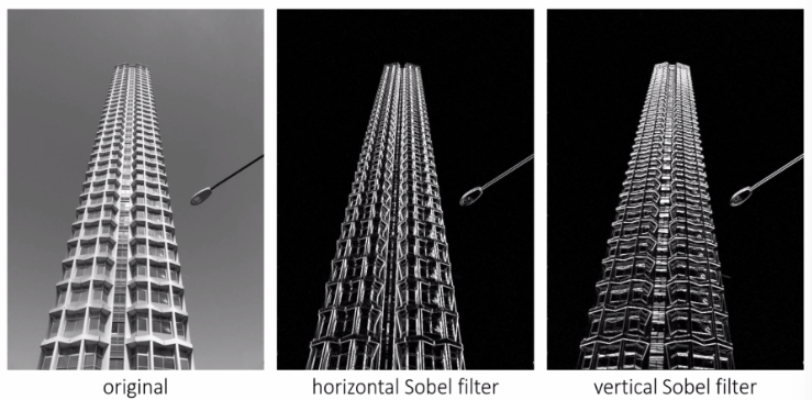
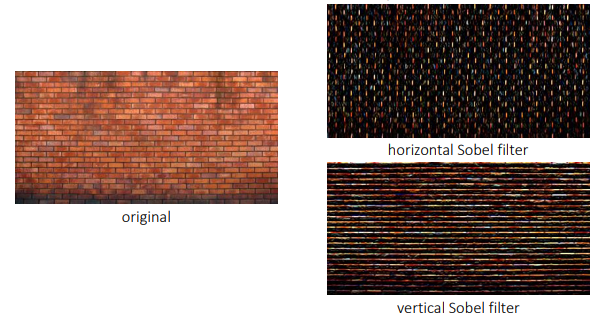
examples

Several Derivative Filters

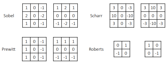
• Sobel 필터(2:1)가 Scharr 필터(10:3)보다 blur ↑
• Roberts Filter: 대각선으로 검출

Computing Image gradients

1. 미분 필터 선택 (sobel, scharr, ...)
2. convolution 진행
3. 이미지 gradient 구성 + 방향 & 크기 계산

Gradient
기울기를 vector로 나타냄

Direction
기울기 방향 확인

Amplitude
기울기 크기 절대값으로 변환

How do you find the edge of this signal?

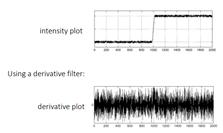
노이즈가 많으면 제대로 edge를 검출할 수 없음

• 비어있는 부분은 이웃(neighbor) 없는 애들
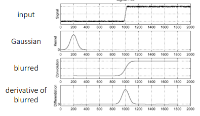
• 얼마만큼을 blur할지 적정점 찾는 것이 중요

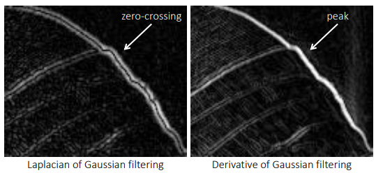
DoG Filter

Derivative of Gaussian Filter

$f$ : 기존 이미지
$h$ : 가우시안 필터

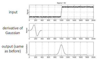
(기존 이미지 x 가우시안 필터)를 미분 → 기존이미지 x (가우시안 필터를 미분한 것)

원래 방식: $O(2n^2m^2)$
개선된 방식: $O(n^2m^2)$

▶ 더 효율적 + 더 빠름

Laplace Filter

2차 미분 필터

1차 미분

2차 미분

$g(x) = f'(x)$라고 볼때,

여기서, $f'(x+0.5h)$는,

$f'(x-0.5h)$도 마찬가지로,

따라서,

LoG Filter

Laplacian of Gaussian Filter

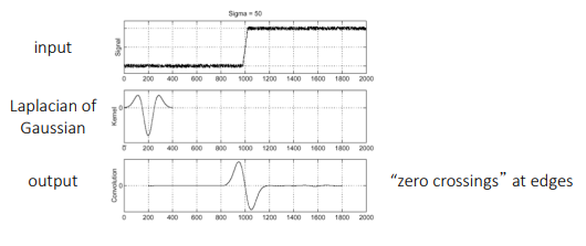
LoG vs DoG

2D 가우시안 필터