Ch.2 Image Pyramids & Frequency domain
Image Downsampling
Naive Image Downsampling
im[::2, ::2] → 한 픽셀씩 건너뛰기
▶ 해상도↓ 정보량↓ (=aliasing)
Aliasing
현실: 연속
이미지: discrete (or) sampled 된 현실
discrete (이산): 구별되고 별개의 값이나 상태를 가진 표현
→ (컴퓨터비전) 디지털 이미지의 픽셀값
sample (샘플): 특정 간격으로 연속 신호나 장면의 측정값을 취하여 표현
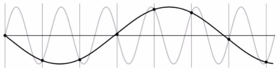
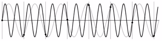
Sampling
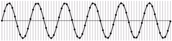
Under-sampling
정보의 손실:
더 낮은 주파수의 신호로 잘못 파악할 수 있다.note
(언제나) 더 높은 주파수의 신호로 잘못 파악할 수 있다.
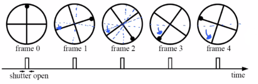
Temporal Aliasing
Anti-Aliasing
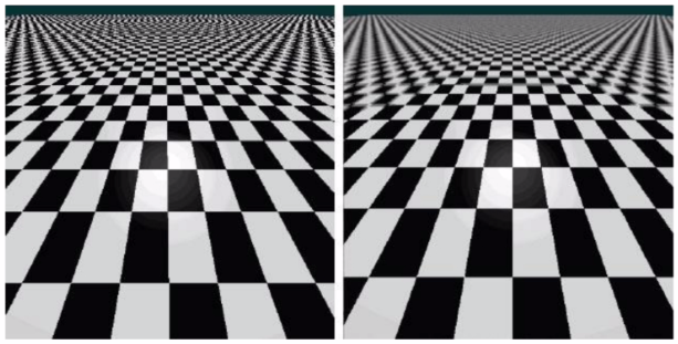
안티-에일리어싱 방법
1. over-sampling samples
2. 먼저 blur하고, 이후 샘플링
2번 방법
보통 가우시안 필터 사용주파수↓ & 디테일↓ (정보가 손실되긴 함)
▶ 샘플링 덜 해도 괜찮아짐Q1.
얼마나 blur 해야할까?Q2.
얼마 단위로 샘플링 해야할까?A.
Nyquist limit에 도달할 때까지
Gaussian Image Pyramid
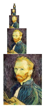
길이: , 넓이: → 길이: , 넓이: → ...
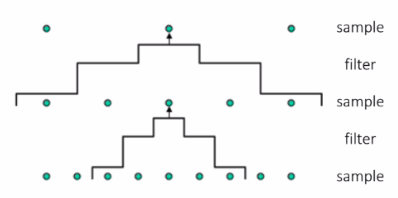
Constructing a Gaussian Pyramid
algorithm
repeat:
  filter
  subsample
(until min resolution reached)
Q.
전체 피라미드의 크기
A.
height:
area:
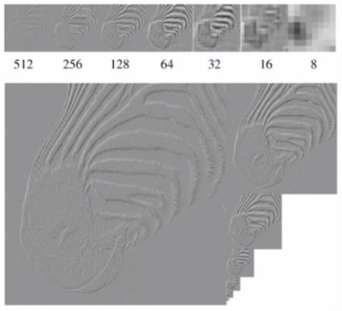
Some properties of the Gaussian pyramid
레벨이 높아질수록 blur (정보 손실됨)
→ 큰 디테일만 남음
▶ 더 높은 레벨로 복원 (upsampling) 불가능
Blurring is lossy
Residual 남겨두면 다시 업샘플링 가능
- downsampling 해버리면 차원이 되어버려 연산(-) 불가능
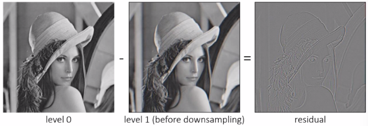
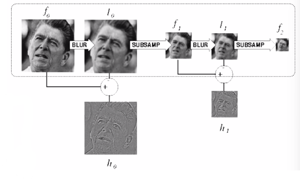
Laplacian Image Pyramid
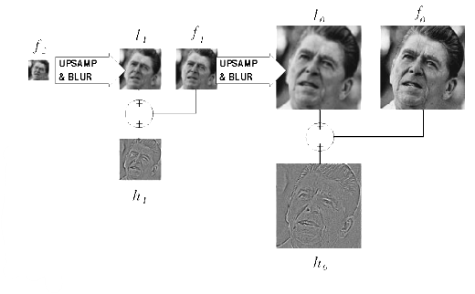
Residual & 가장 윗 level 이미지 가지고 있으면 원본 이미지 복원 가능
bit 개수↓ & 값의 range 훨씬 적음
▶ 압축률↑
Constructing a Laplacian Pyramid
algorithm
repeat:
  filter
  compute residual
  subsample
(until min resolution reached)
Reconstructing the original image
algorithm
repeat:
  upsample
  sum with residual
(until original resolution reached)
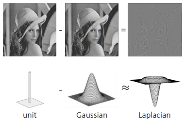
Why is it called a Laplacian Pyramid?
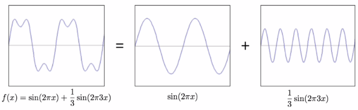
Fourier Series
Basic building block
사인파 함수
: 진폭
- 주파수의 높이
: 각주파수
- 시간 단위 Hz 내에서 사인파의 완전한 주기 횟수 - 속도 or 밀도)
- (: 사인파의 주파수)
: 위상이동
- 원래 위치()일때, 수평으로 얼마나 이동하는지
- 양의 위상이동: 사인파를 왼쪽으로 이동시킴
- 음의 위상이동: 사인파를 오른쪽으로 이동시킴
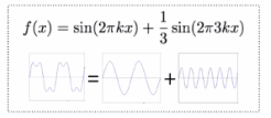
Examples
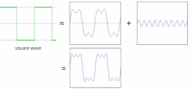
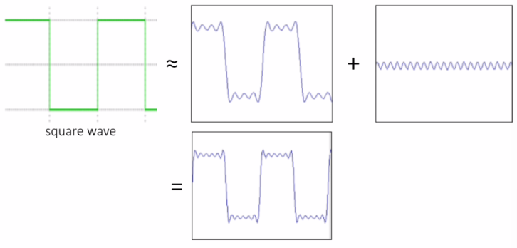
square wave
Frequency Domain
Visualizing the frequency spectrum
| 주파수 | ||
| 증폭 |
Examples
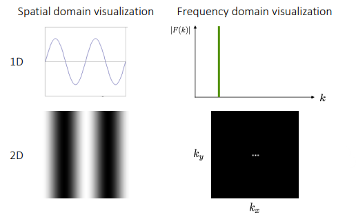
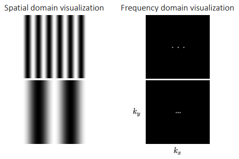
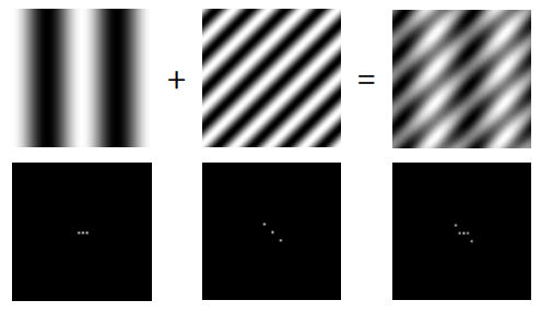
- 주파수: 계속 더해도 사라지지 않음.
Fourier Transform
Recalling some basics
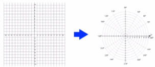
Rectangular Coordinates
: 실수 부분
: 허수 부분
▼
Alternative Reparameterization
▼
극 좌표계 (polar coordinates)
▼
(polar transform)
▼
지수 표기법 (exponential form)
▼
(오일러 공식)
▼
Fourier Transform
Fourier Transform - continuous
Inverse Fourier Transform - continuous
Fourier Transform - discrete
Inverse Fourier Transform - discrete
Connection to the 'Summation of Sine Waves' idea
▼
오일러 공식
▼
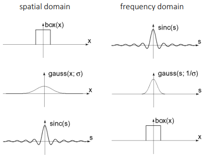
Fourier Transform Pairs
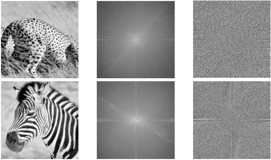
Fourier transform of natural images
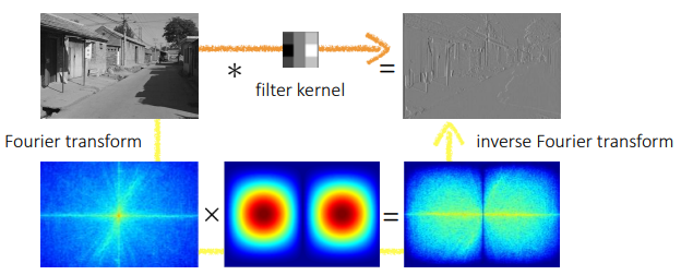
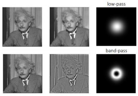
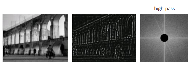
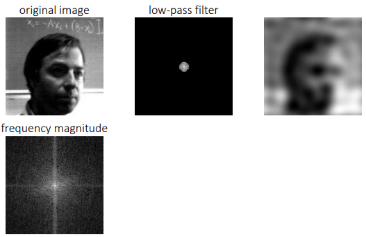
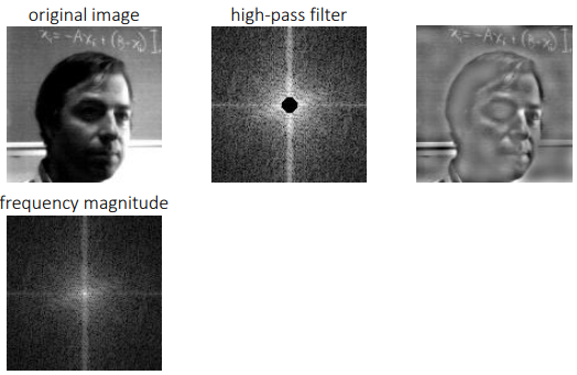
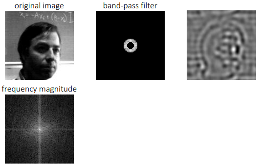
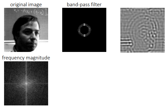
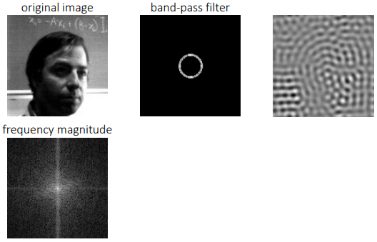
Frequency-Domain Filtering
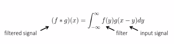
The convolution theorem
-
두 함수의 convolution의 푸리에변환 = 각 함수의 푸리에 변환의 곱
-
inverse도 마찬가지
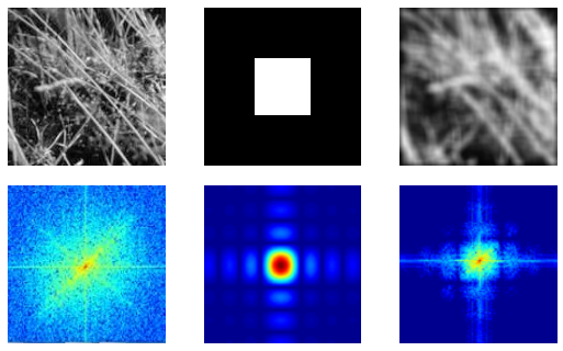
Spatial domain filtering
가우시안 Blur
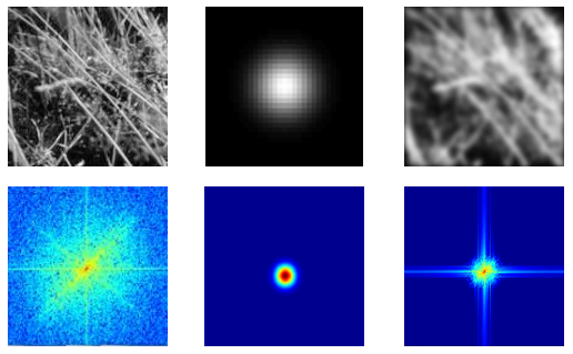
Box Blur
More filtering examples

Revisiting Sampling
The Nyquist-Shannon sampling theorem
minimum: 6Hz,
▶ 6Hz ↑ : aliasing X
▶ 6Hz ↓ : aliasing O
