[kaggle/python] House Price prediction

📌 주제: House Price prediction

📖 참고 솔루션

Stacked Regressions : Top 4% on LeaderBoard(by Serigne)

---

✔️ Understand the problem

⚡ 변수, 데이터셋 살펴보기

✏️ 필요한 라이브러리 불러오기

# 라이브러리 불러오기
import numpy as np
import pandas as pd             # data processing, CSV file I/O
import matplotlib.pyplot as plt
%matplotlib inline
import seaborn as sns
color = sns.color_palette()
sns.set_style('darkgrid')

import warnings
def ignore_warn(*args, **kwargs):
    pass
warnings.warn = ignore_warn     #ignore annoying warning (from sklearn and seaborn)

from scipy import stats
from scipy.stats import norm, skew      # for some statistics

pd.set_option('display.float_format', lambda x: '{:.3f}'.format(x))
#Limiting floats output to 3 decimal points

✏️ 데이터셋 가져오기

# 데이터셋 가져오기
train_data = 'C:\\Users\\USER\\Desktop\\Data Analysis\\data\\train2.csv'
test_data = 'C:\\Users\\USER\\Desktop\\Data Analysis\\data\\test2.csv'
train = pd.read_csv(train_data)
test = pd.read_csv(test_data)

✏️ 데이터 확인하기

train.head(5)

✏️ 필요 없는 컬럼(Id) 제거하기

# Id 컬럼을 제거하기 전 sample, feature의 개수 확인하기
print("The train data size before dropping Id feature is : {} ".format(train.shape))
print("The test data size before dropping Id feature is : {} ".format(test.shape))

# Id 컬럼 저장하기
train_ID = train['Id']
test_ID = test['Id']

# Id 컬럼 제거하기
train.drop("Id", axis=1, inplace=True)
test.drop("Id", axis=1, inplace=True)

# Id 컬럼을 제거한 후 sample, feature의 개수 확인하기
print("\nThe train data size before dropping Id feature is : {} ".format(train.shape))
print("The test data size before dropping Id feature is : {} ".format(test.shape))

The train data size before dropping Id feature is : (1460, 81) 
The test data size before dropping Id feature is : (1459, 80) 

The train data size before dropping Id feature is : (1460, 80) 
The test data size before dropping Id feature is : (1459, 79) 

---

✔️ Data Processing

⚡ Outliers

✏️ outlier 확인하기

fig, ax = plt.subplots()
ax.scatter(x = train['GrLivArea'], y = train['SalePrice'])
plt.ylabel('SalePrice', fontsize=13)
plt.xlabel('GrLivArea', fontsize=13)
plt.show()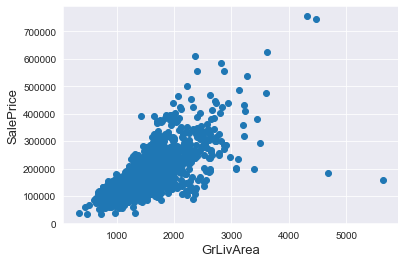

• 그래프의 오른쪽 아래에 위치한 2개의 점을 outlier로 판단하고 제거함

• 그래프의 오른쪽 위에 위치한 2개의 점은 trend를 따르고 있으므로, 제거하지 않음

  ---

  ✏️ outlier 제거하기

train = train.drop(train[(train['GrLivArea'] > 4000) & (train['SalePrice'] < 300000)].index)

# 그래프 확인하기
fig, ax = plt.subplots()
ax.scatter(x = train['GrLivArea'], y = train['SalePrice'])
plt.ylabel('SalePrice', fontsize=13)
plt.xlabel('GrLivArea', fontsize=13)
plt.show()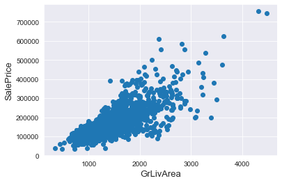

---

⚡ Target Variable (SalePrice)

✏️ normality 확인하기

# Target Variable (SalePrice)
sns.distplot(train['SalePrice'] , fit=norm);

# Get the fitted parameters used by the function
(mu, sigma) = norm.fit(train['SalePrice'])
print( '\n mu = {:.2f} and sigma = {:.2f}\n'.format(mu, sigma))

# Plot the distribution
plt.legend(['Normal dist. ($\mu=$ {:.2f} and $\sigma=$ {:.2f} )'.format(mu, sigma)],
            loc='best')
plt.ylabel('Frequency')
plt.title('SalePrice distribution')

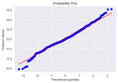
# QQ-plot
fig = plt.figure()
res = stats.probplot(train['SalePrice'], plot=plt)
plt.show()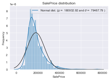

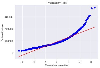
• target variable이 오른쪽으로 skewed되어 있음.

  ---

✏️ 로그변환

# 로그변환 -> numpy fuction log1p을 사용함 -> log(1+x) 적용
train['SalePrice'] = np.log1p(train['SalePrice'])

# 로그변환 후 분포 확인하기
sns.distplot(train['SalePrice'] , fit=norm);

# Get the fitted parameters used by the function
(mu, sigma) = norm.fit(train['SalePrice'])
print( '\n mu = {:.2f} and sigma = {:.2f}\n'.format(mu, sigma))

# Plot the distribution
plt.legend(['Normal dist. ($\mu=$ {:.2f} and $\sigma=$ {:.2f} )'.format(mu, sigma)],
            loc='best')
plt.ylabel('Frequency')
plt.title('SalePrice distribution')

# QQ-plot
fig = plt.figure()
res = stats.probplot(train['SalePrice'], plot=plt)
plt.show()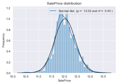

---

⚡ Features engineering

✏️ train data와 test data를 동일한 데이터프레임으로 연결하기

ntrain = train.shape[0]     # 행의 수(1458)
ntest = test.shape[0]       # 행의 수(1459)
y_train = train.SalePrice.values
all_data = pd.concat((train, test)).reset_index(drop=True)
all_data.drop(['SalePrice'], axis=1, inplace=True)
print("all_data size is : {}".format(all_data.shape))

all_data size is : (2917, 79)

✏️ missing data

all_data_na = (all_data.isnull().sum() / len(all_data)) * 100
all_data_na = all_data_na.drop(all_data_na[all_data_na == 0].index).sort_values(ascending=False)[:30]
# missing value가 존재하지 않는 컬럼은 drop
missing_data = pd.DataFrame({'Missing Ratio' : all_data_na})
missing_data.head(20)

	Missing Ratio
PoolQC	99.691
MiscFeature	96.400
Alley	93.212
Fence	80.425
FireplaceQu	48.680
LotFrontage	16.661
GarageFinish	5.451
GarageQual	5.451
GarageCond	5.451
…	…

# 시각화
f, ax = plt.subplots(figsize=(15,12))
plt.xticks(rotation='90')
sns.barplot(x=all_data_na.index, y=all_data_na)     # x: features, y: missing ratio
plt.xlabel('Features', fontsize=15)
plt.ylabel('Percent of missing values', fontsize=15)
plt.title('Percent missing data by feature', fontsize=15)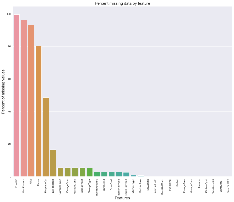

---

✏️ Data correlation

corrmat = train.corr()
plt.subplots(figsize=(12,9))
sns.heatmap(corrmat, vmax=0.9, square=True)

✏️ Imputing missing values

• NaN 값을 "None"으로 치환

all_data['PoolQC'] = all_data['PoolQC'].fillna("None") 
all_data['MiscFeature'] = all_data['MiscFeature'].fillna("None")
all_data['MiscFeature'] = all_data['MiscFeature'].fillna("None")
all_data['Alley'] = all_data['Alley'].fillna("None")
all_data['Fence'] = all_data['Fence'].fillna("None")
all_data['FireplaceQu'] = all_data['FireplaceQu'].fillna("None")
all_data["MasVnrType"] = all_data["MasVnrType"].fillna("None")

for col in ('BsmtQual', 'BsmtCond', 'BsmtExposure', 'BsmtFinType1', 'BsmtFinType2'):
    all_data[col] = all_data[col].fillna('None')

all_data['MSSubClass'] = all_data['MSSubClass'].fillna("None")

• missing value를 중앙값으로 치환

all_data["LotFrontage"] = all_data.groupby("Neighborhood")["LotFrontage"].transform(
    lambda x: x.fillna(x.median()))

• 결측값을 0으로 치환

for col in ('GarageYrBlt', 'GarageArea', 'GarageCars'):
    all_data[col] = all_data[col].fillna(0)

for col in ('BsmtFinSF1', 'BsmtFinSF2', 'BsmtUnfSF','TotalBsmtSF', 'BsmtFullBath', 'BsmtHalfBath'):
    all_data[col] = all_data[col].fillna(0)

all_data["MasVnrArea"] = all_data["MasVnrArea"].fillna(0)

• 결측값을 최빈값으로 치환

all_data['MSZoning'] = all_data['MSZoning'].fillna(all_data['MSZoning'].mode()[0])
all_data['Electrical'] = all_data['Electrical'].fillna(all_data['Electrical'].mode()[0])
all_data['KitchenQual'] = all_data['KitchenQual'].fillna(all_data['KitchenQual'].mode()[0])
all_data['Exterior1st'] = all_data['Exterior1st'].fillna(all_data['Exterior1st'].mode()[0])
all_data['Exterior2nd'] = all_data['Exterior2nd'].fillna(all_data['Exterior2nd'].mode()[0])
all_data['SaleType'] = all_data['SaleType'].fillna(all_data['SaleType'].mode()[0])

• Utilities 컬럼 제거

all_data = all_data.drop(['Utilities'], axis=1)

• 'Typ'로 치환

all_data['Functional'] = all_data['Functional'].fillna('Typ')

---

✏️ 남은 결측값이 있는지 확인하기

all_data_na = (all_data.isnull().sum() / len(all_data)) * 100
all_data_na = all_data_na.drop(all_data_na[all_data_na == 0].index).sort_values(ascending=False)
missing_data = pd.DataFrame({'Missing Ratio' :all_data_na})
missing_data.head()

• missing value가 더 이상 존재하지 않음.

---

✏️ 데이터타입 변경하기

• numerical variable의 데이터타입 변경

all_data['MSSubClass'] = all_data['MSSubClass'].apply(str)
all_data['MSSubClass']

• categorical하게 변경

all_data['OverallCond'] = all_data['OverallCond'].astype(str)
all_data['OverallCond']

all_data['YrSold'] = all_data['YrSold'].astype(str)
all_data['MoSold'] = all_data['MoSold'].astype(str)

• LabelEncoder: Categorical 데이터를 Numerical로 변환

from sklearn.preprocessing import LabelEncoder
cols = ('FireplaceQu', 'BsmtQual', 'BsmtCond', 'GarageQual', 'GarageCond', 
        'ExterQual', 'ExterCond','HeatingQC', 'PoolQC', 'KitchenQual', 'BsmtFinType1', 
        'BsmtFinType2', 'Functional', 'Fence', 'BsmtExposure', 'GarageFinish', 'LandSlope',
        'LotShape', 'PavedDrive', 'Street', 'Alley', 'CentralAir', 'MSSubClass', 'OverallCond', 
        'YrSold', 'MoSold')

# process columns, apply LabelEncoder to categorical features
for c in cols:
    lbl = LabelEncoder()
    lbl.fit(list(all_data[c].values))
    all_data[c] = lbl.transform(list(all_data[c].values))

# shape
print('Shape all_data: {}'.format(all_data.shape))

Shape all_data: (2917, 78)

---

✏️ 새로운 변수 생성하기

• 지하실, 1층, 2층의 area를 합한 새로운 변수 생성

all_data['TotalSF'] = all_data['TotalBsmtSF'] + all_data['1stFlrSF'] + all_data['2ndFlrSF']

---

✏️ Skewed features 확인하기

numeric_feats = all_data.dtypes[all_data.dtypes != "object"].index      # 문자열이 아닌 변수만

skewed_feats = all_data[numeric_feats].apply(lambda x: skew(x.dropna())).sort_values(ascending=False)
# apply: 행 방향 또는 열 방향으로 지정한 함수 적용
# apply(lambda 입력값: 결과값)
# skew(): 왜도 계산
# dropna(): 결측값이 있는 row을 drop함
print("\nSkew in numerical features: \n")
skewness = pd.DataFrame({'Skew' : skewed_feats})
skewness.head(10)

	Skew
MiscVal	21.940
PoolArea	17.689
LotArea	13.109
LowQualFinSF	12.085
3SsnPorch	11.372
LandSlope	4.973
KitchenAbvGr	4.301
BsmtFinSF2	4.145
EnclosedPorch	4.002
ScreenPorch	3.945

---

✏️ Box-Cox transformation

# Box-Cox transformation -> lambda=0 이면 로그변환과 동일
# boxcox1p -> x가 아닌 (1+x)가 들어감. 만약 lambda=0 이면 log(1+x)가 적용되므로 이는 log1p와 같음
skewness = skewness[abs(skewness) > 0.75]       # skewness > 0.75인 변수
print("There are {} skewed numerical features to Box Cox transform".format(skewness.shape[0]))

from scipy.special import boxcox1p
skewed_features = skewness.index
lam = 0.15
for feat in skewed_features:
    all_data[feat] = boxcox1p(all_data[feat], lam)

There are 59 skewed numerical features to Box Cox 

---

✏️ dummy categorical features

all_data = pd.get_dummies(all_data)
print(all_data.shape)

• Getting the new train and test sets

train = all_data[:ntrain]       # 1458행(0~1457)
test = all_data[ntrain:]        # 1459행(1458~2916)

---

✔️ Modelling

# 라이브러리 불러오기
from sklearn.linear_model import ElasticNet, Lasso,  BayesianRidge, LassoLarsIC
from sklearn.ensemble import RandomForestRegressor,  GradientBoostingRegressor
from sklearn.kernel_ridge import KernelRidge
from sklearn.pipeline import make_pipeline
from sklearn.preprocessing import RobustScaler
from sklearn.base import BaseEstimator, TransformerMixin, RegressorMixin, clone
from sklearn.model_selection import KFold, cross_val_score, train_test_split
from sklearn.metrics import mean_squared_error
import xgboost as xgb
import lightgbm as lgb

✏️ Validation function

n_folds = 5

def rmsle_cv(model):
    kf = KFold(n_folds, shuffle=True, random_state=42).get_n_splits(train.values)
    rmse = np.sqrt(-cross_val_score(model, train.values, y_train, scoring="neg_mean_squared_error", cv=kf))
    return(rmse)

---

⚡ Base models

LASSO Regression

lasso = make_pipeline(RobustScaler(), Lasso(alpha=0.0005, random_state=1))

Elastic-Net Regression

ENet = make_pipeline(RobustScaler(), ElasticNet(alpha=0.0005, l1_ratio=.9, random_state=3))

Kernel Ridge Regression

KRR = KernelRidge(alpha=0.6, kernel='polynomial', degree=2, coef0=2.5)

Gradient Boosting Regression

GBoost = GradientBoostingRegressor(n_estimators=3000, learning_rate=0.05, max_depth=4, max_features='sqrt', min_samples_leaf=15, min_samples_split=10, loss='huber', random_state=5)

XGBoost

model_xgb = xgb.XGBRegressor(colsample_bytree=0.4603, gamma=0.0468, learning_rate=0.05, max_depth=3, min_child_weight=1.7817, n_estimators=2200, reg_alpha=0.4640, reg_lambda=0.8571, subsample=0.5213, silent=1, random_state=7, nthread=-1)

• colsample_bytree: 각 트리별 feature의 샘플링 비율, learning_rate: 가중치
• min_child_weight: 관측치에 대한 가중치 합의 최소값, n_estimators: 생성할 weak learner의 수

LightGBM

model_lgb = lgb.LGBMRegressor(objective='regression', num_leaves=5, learning_rate=0.05, n_estimators=720, max_bin=55, bagging_fraction=0.8, bagging_freq=5, feature_fraction=0.2319, feature_fration_seed=9, bagging_seed=9, min_data_in_leaf=6, min_sum_hessian_in_leaf=11)

---

✏️ base models score

score: LASSO

score = rmsle_cv(lasso)
print("\nLasso score: {:.4f} ({:.4f})\n".format(score.mean(), score.std()))

Lasso score: 0.1115 (0.0074)

score: Elastic-Net

score = rmsle_cv(ENet)
print("ElasticNet score: {:.4f} ({:.4f})\n".format(score.mean(), score.std()))

ElasticNet score: 0.1116 (0.0074)

score: Kernel Ridge Regression

score = rmsle_cv(KRR)
print("Kernel Ridge score: {:.4f} ({:.4f})\n".format(score.mean(), score.std()))

Kernel Ridge score: 0.1153 (0.0075)

score: Gradient Boosting Regression

score = rmsle_cv(GBoost)
print("Gradient Boosting score: {:.4f} ({:.4f})\n".format(score.mean(), score.std()))

Gradient Boosting score: 0.1167 (0.0083)

score: XGBoost

score = rmsle_cv(model_xgb)
print("Xgboost score: {:.4f} ({:.4f})\n".format(score.mean(), score.std()))

Xgboost score: 0.1164 (0.0070)

score: LightGBM

score = rmsle_cv(model_lgb)
print("LGBM score: {:.4f} ({:.4f})\n" .format(score.mean(), score.std()))

LGBM score: 0.1160 (0.0064)

---

⚡ Stacking models

✏️ Simplest Stacking approach : Averaging base models

# Average base models class
class AveragingModels(BaseEstimator, RegressorMixin, TransformerMixin):
    def __init__(self, models):
        self.models = models
        
    # we define clones of the original models to fit the data in
    def fit(self, X, y):
        self.models_ = [clone(x) for x in self.models]
        
        # Train cloned base models
        for model in self.models_:
            model.fit(X, y)

        return self
    
    #Now we do the predictions for cloned models and average them
    def predict(self, X):
        predictions = np.column_stack([
            model.predict(X) for model in self.models_
        ])
        return np.mean(predictions, axis=1)

---

✏️ Averaged base models score: ENet, GBoost, KRR, Lasso

averaged_models = AveragingModels(models = (ENet, GBoost, KRR, lasso))

score = rmsle_cv(averaged_models)
print(" Averaged base models score: {:.4f} ({:.4f})\n".format(score.mean(), score.std()))

 Averaged base models score: 0.1087 (0.0077)

---

✏️ Less simple Stacking : Adding a Meta-model

# Stacking averaged Models Class
class StackingAveragedModels(BaseEstimator, RegressorMixin, TransformerMixin):
    def __init__(self, base_models, meta_model, n_folds=5):
        self.base_models = base_models
        self.meta_model = meta_model
        self.n_folds = n_folds
   
    # We again fit the data on clones of the original models
    def fit(self, X, y):
        self.base_models_ = [list() for x in self.base_models]
        self.meta_model_ = clone(self.meta_model)
        kfold = KFold(n_splits=self.n_folds, shuffle=True, random_state=156)
        
        # Train cloned base models then create out-of-fold predictions
        # that are needed to train the cloned meta-model
        out_of_fold_predictions = np.zeros((X.shape[0], len(self.base_models)))
        for i, model in enumerate(self.base_models):
            for train_index, holdout_index in kfold.split(X, y):
                instance = clone(model)
                self.base_models_[i].append(instance)
                instance.fit(X[train_index], y[train_index])
                y_pred = instance.predict(X[holdout_index])
                out_of_fold_predictions[holdout_index, i] = y_pred
        
        # Now train the cloned  meta-model using the out-of-fold predictions as new feature
        self.meta_model_.fit(out_of_fold_predictions, y)
        return self
    
    #Do the predictions of all base models on the test data and use the averaged predictions as 
    #meta-features for the final prediction which is done by the meta-model
    def predict(self, X):
        meta_features = np.column_stack([
            np.column_stack([model.predict(X) for model in base_models]).mean(axis=1)
            for base_models in self.base_models_ ])
        return self.meta_model_.predict(meta_features)
    

---

✏️ Stacking Averaged models Score

stacked_averaged_models = StackingAveragedModels(base_models = (ENet, GBoost, KRR), meta_model = lasso)

score = rmsle_cv(stacked_averaged_models)
print("Stacking Averaged models score: {:.4f} ({:.4f})".format(score.mean(), score.std()))

Stacking Averaged models score: 0.1081 (0.0073)

---

✏️ Ensembling StackedRegressor, XGBoost and LightGBM*

rmsle evaluation function

def rmsle(y, y_pred):
    return np.sqrt(mean_squared_error(y, y_pred))

StackedRegressor

stacked_averaged_models.fit(train.values, y_train)
stacked_train_pred = stacked_averaged_models.predict(train.values)
stacked_pred = np.expm1(stacked_averaged_models.predict(test.values))
print(rmsle(y_train, stacked_train_pred))

0.07839506096666397

• np.expm1: 각 요소에 자연상수를 밑으로 하는 지수함수를 적용한 뒤, 1을 뺀 것
  -> f(x) = e^x - 1

XGBoost

model_xgb.fit(train, y_train)
xgb_train_pred = model_xgb.predict(train)
xgb_pred = np.expm1(model_xgb.predict(test))
print(rmsle(y_train, xgb_train_pred))

0.07876050033097799

LightGBM

model_lgb.fit(train, y_train)
lgb_train_pred = model_lgb.predict(train)
lgb_pred = np.expm1(model_lgb.predict(test.values))
print(rmsle(y_train, lgb_train_pred))

0.07255428955736014

---

# RMSE on the entire Train data when averaging
print('RMSLE score on train data:')
print(rmsle(y_train,stacked_train_pred*0.70 +
               xgb_train_pred*0.15 + lgb_train_pred*0.15 ))

---

✏️ Ensemble prediction

ensemble = stacked_pred*0.70 + xgb_pred*0.15 + lgb_pred*0.15
ensemble