0. 핵심개념 및 사이킷런 알고리즘 API 링크
sklearn.cluster.KMeans
1. Clustering 이해
import warnings
warnings.filterwarnings("ignore")
import numpy as np
import pandas as pd
import matplotlib.pyplot as plt
plt.style.use('seaborn-deep')
import matplotlib.cm
cmap = matplotlib.cm.get_cmap('plasma')
from sklearn.cluster import KMeans
data = pd.read_csv('Mall_Customers.csv')
X = data.iloc[:, [3,4]]
X.head()
Income Spend
0 15 39
1 15 81
2 16 6
3 16 77
4 17 40
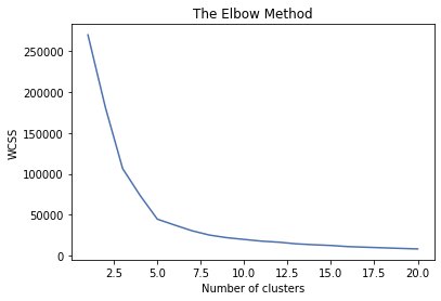
wcss = []
for i in range(1,21):
kmeans = KMeans(n_clusters=i)
kmeans.fit_transform(X)
wcss.append(kmeans.inertia_)
wcss
[269981.28000000014,
181665.82312925166,
106348.37306211119,
73679.78903948837,
44448.45544793369,
37239.83554245604,
30259.657207285458,
25018.576334776328,
21818.11458845217,
19664.68519600554,
17595.28888108518,
16286.850886958873,
14300.044641632878,
13167.778522689903,
12283.892784992784,
10853.593442084231,
10156.765398731703,
9410.284737974447,
8708.406236275801,
8039.671850613157]
plt.figure()
plt.plot(range(1,21), wcss)
plt.title('The Elbow Method')
plt.xlabel('Number of clusters')
plt.ylabel('WCSS')
plt.show()
k = 5
kmeans = KMeans(n_clusters = k)
y_kmeans = kmeans.fit_predict(X)
y_kmeans
array([1, 2, 1, 2, 1, 2, 1, 2, 1, 2, 1, 2, 1, 2, 1, 2, 1, 2, 1, 2, 1, 2,
1, 2, 1, 2, 1, 2, 1, 2, 1, 2, 1, 2, 1, 2, 1, 2, 1, 2, 1, 2, 1, 3,
1, 2, 3, 3, 3, 3, 3, 3, 3, 3, 3, 3, 3, 3, 3, 3, 3, 3, 3, 3, 3, 3,
3, 3, 3, 3, 3, 3, 3, 3, 3, 3, 3, 3, 3, 3, 3, 3, 3, 3, 3, 3, 3, 3,
3, 3, 3, 3, 3, 3, 3, 3, 3, 3, 3, 3, 3, 3, 3, 3, 3, 3, 3, 3, 3, 3,
3, 3, 3, 3, 3, 3, 3, 3, 3, 3, 3, 3, 3, 4, 0, 4, 3, 4, 0, 4, 0, 4,
3, 4, 0, 4, 0, 4, 0, 4, 0, 4, 3, 4, 0, 4, 0, 4, 0, 4, 0, 4, 0, 4,
0, 4, 0, 4, 0, 4, 0, 4, 0, 4, 0, 4, 0, 4, 0, 4, 0, 4, 0, 4, 0, 4,
0, 4, 0, 4, 0, 4, 0, 4, 0, 4, 0, 4, 0, 4, 0, 4, 0, 4, 0, 4, 0, 4,
0, 4])
Group_cluster=pd.DataFrame(y_kmeans)
Group_cluster.columns=['Group']
full_data=pd.concat([data, Group_cluster], axis=1)
full_data
ID Gender Age Income Spend Group
0 1 Male 19 15 39 1
1 2 Male 21 15 81 2
2 3 Female 20 16 6 1
3 4 Female 23 16 77 2
4 5 Female 31 17 40 1
... ... ... ... ... ... ...
195 196 Female 35 120 79 4
196 197 Female 45 126 28 0
197 198 Male 32 126 74 4
198 199 Male 32 137 18 0
199 200 Male 30 137 83 4
200 rows × 6 columns
kmeans_pred = KMeans(n_clusters=k, random_state=42).fit(X)
kmeans_pred.cluster_centers_
array([[55.2962963 , 49.51851852],
[88.2 , 17.11428571],
[26.30434783, 20.91304348],
[25.72727273, 79.36363636],
[86.53846154, 82.12820513]])
kmeans_pred.predict([[100, 50], [30, 80]])
array([4, 3])
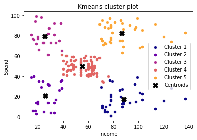
labels = [('Cluster ' + str(i+1)) for i in range(k)]
labels
['Cluster 1', 'Cluster 2', 'Cluster 3', 'Cluster 4', 'Cluster 5']
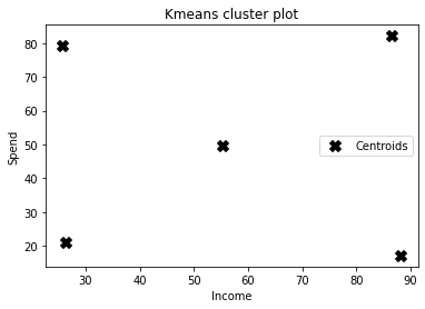
X=np.array(X)
plt.figure()
for i in range(k):
plt.scatter(X[y_kmeans == i, 0], X[y_kmeans == i, 1], s = 20,
c = cmap(i/k), label = labels[i])
plt.scatter(kmeans.cluster_centers_[:,0], kmeans.cluster_centers_[:,1],
            s = 100, c = 'black', label = 'Centroids', marker = 'X')
plt.xlabel('Income')
plt.ylabel('Spend')
plt.title('Kmeans cluster plot')
plt.legend()
plt.show()
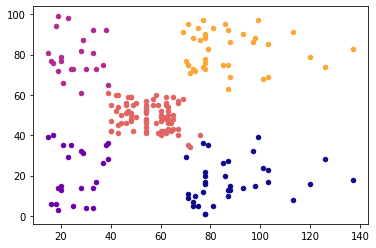
plt.figure()
for i in range(k):
    plt.scatter(X[y_kmeans == i, 0], X[y_kmeans == i, 1], s = 20,
                 c = cmap(i/k), label = labels[i])
plt.scatter(kmeans.cluster_centers_[:,0], kmeans.cluster_centers_[:,1],
            s = 100, c = 'black', label = 'Centroids', marker = 'X')
plt.xlabel('Income')
plt.ylabel('Spend')
plt.title('Kmeans cluster plot')
plt.legend()
plt.show()
2. k-mean Clustering
from scipy.spatial.distance import cdist, pdist
from sklearn.cluster import KMeans
from sklearn.metrics import silhouette_score
iris = pd.read_csv("iris.csv")
print (iris.head())
sepal_length sepal_width petal_length petal_width class
0 5.1 3.5 1.4 0.2 Iris-setosa
1 4.9 3.0 1.4 0.2 Iris-setosa
2 4.7 3.2 1.3 0.2 Iris-setosa
3 4.6 3.1 1.5 0.2 Iris-setosa
4 5.0 3.6 1.4 0.2 Iris-setosa
x_iris = iris.drop(['class'],axis=1)
y_iris = iris["class"]
x_iris.head()
sepal_length sepal_width petal_length petal_width
0 5.1 3.5 1.4 0.2
1 4.9 3.0 1.4 0.2
2 4.7 3.2 1.3 0.2
3 4.6 3.1 1.5 0.2
4 5.0 3.6 1.4 0.2
y_iris.head()
0 Iris-setosa
1 Iris-setosa
2 Iris-setosa
3 Iris-setosa
4 Iris-setosa
Name: class, dtype: object
x_iris.describe()
sepal_length sepal_width petal_length petal_width
count 150.000000 150.000000 150.000000 150.000000
mean 5.843333 3.054000 3.758667 1.198667
std 0.828066 0.433594 1.764420 0.763161
min 4.300000 2.000000 1.000000 0.100000
25% 5.100000 2.800000 1.600000 0.300000
50% 5.800000 3.000000 4.350000 1.300000
75% 6.400000 3.300000 5.100000 1.800000
max 7.900000 4.400000 6.900000 2.500000
from sklearn.preprocessing import StandardScaler
scale=StandardScaler()
scale.fit(x_iris)
X_scale=scale.transform(x_iris)
pd.DataFrame(X_scale).head()
0 1 2 3
0 -0.900681 1.032057 -1.341272 -1.312977
1 -1.143017 -0.124958 -1.341272 -1.312977
2 -1.385353 0.337848 -1.398138 -1.312977
3 -1.506521 0.106445 -1.284407 -1.312977
4 -1.021849 1.263460 -1.341272 -1.312977
K = range(1,10)
KM = [KMeans(n_clusters=k).fit(X_scale) for k in K]
centroids = [k.cluster_centers_ for k in KM]
D_k = [cdist(x_iris, centrds, 'euclidean') for centrds in centroids]
D_k
array~
cIdx = [np.argmin(D,axis=1) for D in D_k]
dist = [np.min(D,axis=1) for D in D_k]
avgWithinSS = [sum(d)/X_scale.shape[0] for d in dist]
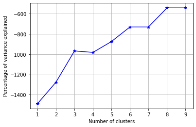
wcss = [sum(d**2) for d in dist]
tss = sum(pdist(X_scale)**2)/X_scale.shape[0]
bss = tss-wcss
fig = plt.figure()
ax = fig.add_subplot(111)
ax.plot(K, avgWithinSS, 'b*-')
plt.grid(True)
plt.xlabel('Number of clusters')
plt.ylabel('Average within-cluster sum of squares')
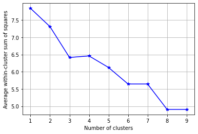
fig = plt.figure()
ax = fig.add_subplot(111)
ax.plot(K, bss/tss*100, 'b*-')
plt.grid(True)
plt.xlabel('Number of clusters')
plt.ylabel('Percentage of variance explained')
import numpy as np
w,v = np.linalg.eig(np.array([[ 0.91335 ,0.75969 ],[ 0.75969,0.69702]]))
print ("\nEigen Values\n",w)
print ("\nEigen Vectors\n",v)
Eigen Values
[1.57253666 0.03783334]
Eigen Vectors
[[ 0.75530088 -0.6553782 ]
[ 0.6553782 0.75530088]]
k_means_fit = KMeans(n_clusters=4, max_iter=300)
k_means_fit.fit(X_scale)
KMeans(n_clusters=4)
k_means_fit.cluster_centers_
array([[-1.34320731, 0.12656736, -1.31407576, -1.30726051],
[-0.01139555, -0.87288504, 0.37688422, 0.31165355],
[-0.73463631, 1.45201075, -1.29704352, -1.21071997],
[ 1.16743407, 0.15377779, 1.00314548, 1.02963256]])
print ("\nK-Means Clustering - Confusion Matrix\n\n",
pd.crosstab(y_iris,k_means_fit.labels_,rownames = ["Actuall"],colnames = ["Predicted"]) )
K-Means Clustering - Confusion Matrix
Predicted 0 1 2 3
Actuall
Iris-setosa 23 0 27 0
Iris-versicolor 0 39 0 11
Iris-virginica 0 17 0 33
print ("\nSilhouette-score: %0.3f" % silhouette_score(x_iris, k_means_fit.labels_, metric='euclidean'))
Silhouette-score: 0.356
for k in range(2,10):
k_means_fitk = KMeans(n_clusters=k,max_iter=300)
k_means_fitk.fit(x_iris)
print ("For K value",k,",Silhouette-score: %0.3f" % silhouette_score(x_iris, k_means_fitk.labels_, metric='euclidean'))
For K value 2 ,Silhouette-score: 0.681
For K value 3 ,Silhouette-score: 0.553
For K value 4 ,Silhouette-score: 0.498
For K value 5 ,Silhouette-score: 0.489
For K value 6 ,Silhouette-score: 0.367
For K value 7 ,Silhouette-score: 0.358
For K value 8 ,Silhouette-score: 0.348
For K value 9 ,Silhouette-score: 0.345
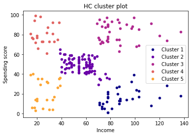
3. Hierarchical Clustering
import numpy as np
import pandas as pd
import matplotlib.pyplot as plt
plt.style.use('seaborn-deep')
import matplotlib.cm
cmap = matplotlib.cm.get_cmap('plasma')
data = pd.read_csv('Mall_Customers.csv')
X = data.iloc[:, [3,4]].values
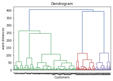
import scipy.cluster.hierarchy as sch
plt.figure(1)
z = sch.linkage(X, method = 'ward')
dendrogram = sch.dendrogram(z)
plt.title('Dendrogram')
plt.xlabel('Customers')
plt.ylabel('ward distances')
plt.show()
k = 5
from sklearn.cluster import AgglomerativeClustering
hc = AgglomerativeClustering(n_clusters = k, affinity = "euclidean", linkage = 'ward')
y_hc = hc.fit_predict(X)
labels = [('Cluster ' + str(i+1)) for i in range(k)]
plt.figure(2)
for i in range(k):
plt.scatter(X[y_hc == i, 0], X[y_hc == i, 1], s = 20,
c = cmap(i/k), label = labels[i])
plt.xlabel('Income')
plt.ylabel('Spending score')
plt.title('HC cluster plot')
plt.legend()
plt.show()