Financial Physics (Econophysics) #1 - Financial Markets as complex systems

Source

• https://users.physics.ox.ac.uk/~Foot/Phynance/

---

Table of Contents

Chapter 1: Financial markets as complex systems

• 1.1 Real problems in finance
• 1.2 Complex systems and Complexity
• 1.3 Financial market overview
• 1.4 Observing the market

---

1. Financial Markets as Complex Systems

1.1. Real Problems in Finance

While pondering the situation and staring at the pricechart, we can’t help but noticing the roller-coaster ride that the stock seems to have had since the IPO. Questions start popping into our heads:

• Does any of that roller-coaster ride in the stock-price x!t" actually tell us anything? If so, what?

• Should we buy (i.e. go long) the stock? Or sell it (i.e. go short)? Maybe we want to use this stock to hedge our risk in other dot-com companies, or in other technology sectors, or in another market.

• What should we then do to minimize our risk? What do we each mean by ‘risk’ – risk of what exactly? Is there any predictability in the stock’s behaviour? How, and to what extent, would such predictability manifest itself on the hourly, daily, or monthly scale?

• Is the roller-coaster ride driven by crowd behaviour? Can we infer what the crowd is thinking? If so, might we then be able to forecast the future based not on the past price series, but on what we believe the crowd will do?

. These questions are however not the types of questions that are easily answered, or even easy to address, within standard finance theory.

Why? Embedded in each of these questions is the issue of $time$, and timing of decisions or actions. Hence in order to really address these questions, we will need to understand something about the time-evolution of the particular asset’s price, and probably also the market in general.

And herein lie the academic and practical motivations for this book: across a broad range of disciplines, researchers are now realizing that some of the hardest problems that they each face have key common elements.

These elements are the key elements of what is now being called a ‘complex’ system. So in order to understand the claim that a financial market is also such a complex system, we will spend a few moments looking at what these key ingredients are.

1.2. Complex Systems and Complexity (복잡계)

Although there is no universally accepted definition of ‘complexity’ or ‘complex system’, most people would agree that any candidate complex
system should have most or all of the following ingredients:

• Feedback: The nature of the feedback can change with time -- for example, becoming positive one moment and negative the next -- and may also change in magnitude and importance. It may operate at the macroscopic or microscopic level, or both. The presence of feedback implies that on some level, buried in the details of the dynamics, the system is ‘remembering’ its past and responding to it, albeit in a highly non-trivial way.

• Non-stationarity: We cannot assume that the dynamical or statistical properties observed in the
  system’s past, will remain unchanged in the system’s future1
  .

• Many interacting agents: The system contains many components or participants, known as ‘agents’, which interact in possibly time-dependent ways. Their individual behaviour will respond to the feedback of information, which is possibly limited, from the system as a whole and/or from other agents. Since these agents may effectively be competing to win, it is unlikely that there is any such thing as a ‘typical’ agent.

• Adaptation: An agent can adapt its behaviour in the hope of improving its performance.

• Evolution: The entire multi-agent population evolves, driven by an ecology of agents who interact and adapt under the influence of feedback. The system typically remains far from equilibrium, and hence can exhibit ‘extreme behaviour’.
  .

• Single realization: The system under study is a single realization, implying that standard techniques whereby averages over time are equated to averages over ensembles, may not work.

• Open system: The system is coupled to the environment, hence it is hard to distinguish between exogenous (i.e. outside) and endogenous (i.e. internal, self-generated) effects.

1.3. Financial Market Overview

1.3.1. The Role of Financial Centres

Examples of financial centres worldwide include London, New
York and Tokyo. Financial centres increasingly find themselves competing in a global marketplace both to retain their domestic market and to win international business. Governments seek to promote their financial centres, not only because of the influx of substantial amounts of foreign capital but also because they provide employment for vast numbers of people.

1.3.2. Types of Financial Market

A distinction is made between primary and secondary markets: a primary market deals in issues of new assets whereas in a secondary market, existing assets are traded.

Liquidity is essentially the freedom to transact assets. Without a liquid secondary market, investors would not be willing to pay as much for new assets on the primary market since they know it would be difficult to sell the assets again.

Vital to the provision of liquidity in the secondary market is the presence of so-called ‘market-makers’. A market-maker will quote buy and sell prices for assets and be willing to accept large trades in either direction in response to market supply and demand.

Secondary markets can have diverse forms in terms of both their macroscopic character and microscopic structure. In ‘screen-based markets’ trading takes place electronically through a (possibly geographically dispersed) IT infrastructure. In a ‘call market’ orders are batched together at infrequent intervals (just once a day in some markets) and a market price is decided by an auction process, either oral or written.

In a ‘continuous market’ prices are quoted continuously by market-makers throughout the trading day. Some markets have a mixture of system.

1.3.3. Financial Assets (skip)

1.3.4. Financial Market Agents (skip)

1.3.5. The Price of an Asset

One of the most important roles of a financial market is to supply, on a continuous basis, a price for a financial asset at which both buyers and sellers are willing to trade.

Classically the ‘value’ of a financial asset is the current value of the total expected future cash flow from that asset. This is the ‘rational expectations’ price of the asset and there are many models in the economics and finance literature for calculating this price (see for example [CLM]).

However, it is an obvious fact that the price of every financial asset moves on a day to day, hour to hour and often second to second basis and that usually there is very little relation between the mean price of the asset and the ‘rational expectations’ price. The question therefore arises as to what determines the price of a financial asset in practice.

1.3.5.1. Role of the Market-maker

We have already discussed the important role of the market-maker in the process of setting a price level for financial assets at which buyers and sellers are willing to trade.

The market-makers supply a willing counterparty for each trade, at a price set by themselves. In the simplest scenario a marketmaker, by contrast to the other market participants, will have no interest in generating a financial return from holding a position in the financial asset and then raising its price.

Ideally, the marketmaker’s manipulation of the price should be solely for the purposes of matching the supply of assets from willing sellers, with the demand for assets from willing buyers. In this way, market-makers can maximize the number of assets traded (i.e. the volume) hence generating market liquidity, and at the same time maximizing their own profit. (Recall that market-makers set a spread between bid and ask prices which generates revenue for them from each traded asset).

In order to pursue our goal of understanding what determines the price level of financial assets in the market, we must therefore answer the question: ‘what determines the demand for assets?’

1.3.5.2. Demand for Assets

We will refer to the number of financial assets sought minus the number offered, as the ‘excess demand’ for the asset. The excess demand, by construction, will be a very complex function of the investors’ beliefs about the asset: in particular, its expected future price levels and its expected future earnings.

These two issues are the principal factors that will be in investors’ minds when they decide to place an order with their broker to buy or sell the asset.

Consequently any realistic model of the excess demand for a financial asset, and hence a model for the asset-price itself, must capture these possible behavioral issues in a very general way.

1.3.6. Orders and Market Clearing

There are different types of request an investor can make of his/her broker. Broadly speaking, investors can place an order with their broker to execute a trade irrespective of the price at which the trade is made, or they can place an order which is dependent on the traded price which can be achieved. We refer to the first (unconditional) type of order as a ‘market order’ and the second (conditional) type as a ‘limit order’.

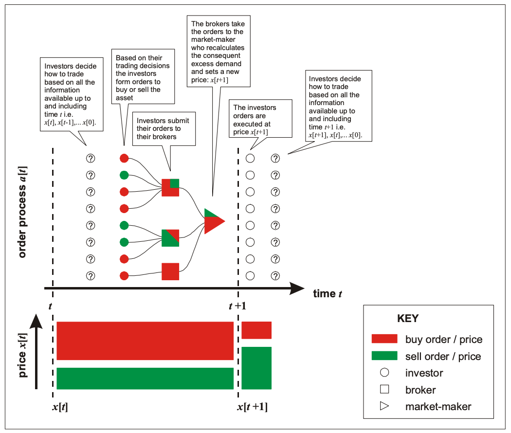
A schematic representation of the temporal order in which events occur in the trading of financial assets through the investor--broker--market-maker chain. For simplicity we assume all orders are market orders and thus are all transacted at the new price set by the market-maker. We also have assumed that all orders are placed at the same time; this is purely for clarity as described in Chapter 4.

the market-maker will execute:

• all market orders
  - all buy orders ($a_i[t, x[t+1]]>0] \: for \: which \: y_i \ge x^{+}[t+1]$)
  - all sell orders ($a_i[t, x[t+1]]<0] \: for \: which \: y_i \le x^{-}[t+1]$)

1.4. Observing the Market

Having given an overview of the inner workings of financial markets, we now step back and assume the position of an outsider who is observing the 'output'. of a particular market.

Despite the large number of variables driving the market itself, as discussed in this Chapter, the outside observer has a very limited number of ouput variables at his disposition. Hence he may be forced to regard the market as a ‘black box’.

For the stock market, the output variables are prices and possibly volumes of trades. In recent years the frequency of the available data has increased enormously: whereas previously only daily prices were disclosed, now it is possible to get trade-by-trade price data (socalled tick-data) albeit with a finite delay time if one doesn’t subscribe to a data provider. Since the price as a function of time $x(t)$" is the primary experimental output variable, or ‘observable’, it is worth discussing it in some detail.

Consider the typical situation in which we, as outsiders, are provided with a set of highfrequency price-data 3x4 over a given, finite time-period.

Linear Price-change

• $\triangle x(t, t-\triangle t) \: = \: x(t) - x(t-\triangle t)$
• $or$ $\triangle x_{t, t-\triangle t} \: = \: x_t - x_{t-\triangle t}$

Discounted or de-trended Price-change

This attempts to remove the effects of inflation or supposedly deterministic bias, etc by introducing a factor $F(t)$.

$\triangle x^{(F)}(t, t-\triangle t) \: = \: F(t)x(t) - F(t-\triangle t)x(t-\triangle t))$

The problem then arises as to what form $F(t)$ should take. Fortunately if $F(t)$ is slowly varying as compared to the time-window over which the data is collected, then we can usually assume

$\triangle x^(F)(t, t-\triangle t) \: \propto \: \triangle x(t, t-\triangle t)$

Return

$R(t, t-\triangle t) \: = \: \frac {x(t)-x(t-\triangle t)}{x(t-\triangle t)}$

Log Return

$z(t, t-\triangle t) \: = \: ln \frac{x(t)}{x(t-\triangle t)} \: = \: ln{x(t)}-ln{x(t-\triangle t)}$

Each of these price-related definitions has its advantages and disadvantages. Any particular choice may or may not bias a given data set, hence confusing the usefulness of the conclusions. Again this is a ractical problem and there is no easy way out, nor is there any ‘right’ and ‘wrong’ answer.

Throughout this book we will switch between these quantities according to the data available, and the problem under consideration. Fortunately these quantities all have similar statistical properties in practice, since the change in price $\triangle x(t-\triangle t)$ is typically small compared to the absolute values $x(t-\triangle t), \: x(t)$.

This reason, combined with the fact that we do not focus on specific stock data, means that we will not tend to worry about the distinction between these various price-change measures in this course.