Asset Pricing and Linear Algebra

허상범·2023년 7월 22일

Finance

목록 보기

7/9

Source

https://doi.org/10.4169/college.math.j.44.1.002

TL;DR & Summary.

Concepts from asset pricing and financial markets theory are used to illustrate concepts of linear algebra and linear programming

Asset Pricing, Financial Markets, and Linear Algebra

The fundamental theorems of asset pricing, for example, provide an opportunity to discuss arbitrage and complete markets.

These are related here to concepts of discrete probability, expected value, linear dependence, and vector basis. Linear programming, i.e., the simplex method, is illustrated by a small-scale problem that can be worked out as a classroom example in optimization courses.

The advanced reader may wish to consult the works of de Finetti [2] and Lad [4] to explore further the fruitful connections between the fundamental theorems of probability and asset pricing.

1. Basic Concepts

1.1. State of the World and State Space

The state of the world is a complete specification of all the relevant events over a specific time horizon.

We work with a finite number of possible states, each denoted
by some ωi, and we refer to $\Omega \: = \: \{\omega_{1}, ... , \omega_{k} \}$ as the state space, the set of all states.

Here we consider only one-period investments, during which period only one state occurs.

1.2. Contingent Claim

Another important concept is contingent claim, a claim for a monetary payment contingent on the specific state of the world.

An example of contingent claim is a share of some company. The owner of the share has the right to receive, for instance, part of the profit of this company. Even a simple bet is a type of contingent claim.

More formally, such a claim can be represented by a k-dimensional vector of payoffs, each element corresponding to the payoff received if the corresponding state occurs.

The return rate of asset $A$ when state $ω_{j}$ occurs is denoted $A_{j}$ .

It is given by the price of the asset after the period—a day, month, or year—divided by its price at the beginning of the period.

A risky asset is an asset whose return is uncertain, i.e., a random variable, since it depends on the state of the world. For instance, suppose asset A pays a return rate of 3% if state 1 occurs, 40% if state 2 happens, −6% if state 3 happens, and 10% when state 4 is observed.

In this case, A1 = 1.03, A2 = 1.4, A3 = 0.94, and A4 = 1.1. We use vector notation and write

$\vec A \: = \: (1.03, 1.4, 0.94, 1.1)$

A probability distribution on states, or probability measure, is denoted by $(p_1, p_2, . . . , p_k)$ , where $p_j$ is the probability that state $j$ happens.

A probability measure is an element of $P$ under given states.

$P = \{(p_1, p_2, \dots , p_k ): 0 ≤ p_j ≤ 1, \sum^k_{j=1}P_{j}=1\}$

Regarding the probability $P$ , the expected return of asset A is

$\forall A, \: E_p[A] \: = \: \sum_{j=1}^{k} A_j p_j$ >

2. Arbitrage

A riskless asset pays a constant return rate, no matter which state of the world happens, that is, there is no uncertainty about its return, meaning that it is not a random variable, but a constant.

All our examples assume the existence of a riskless asset $O$ , whose return rate is denoted by $O_j ≡ r$ .

Usually, it is also assumed that one can borrow or lend money at this riskless rate, just as one can buy or sell risky assets.

Suppose that a risky asset A has a return rate strictly bigger than the riskless rate r no matter which state occurs, that is, $A_j > r, \: for\: j \in (1, k)$

Then any investor can, at the beginning of the period, borrow a dollar from the bank promising to pay a return $r$ , and buy a dollar’s worth of $A$ .

At the end of the period he would get $A_j$ , and after paying $r$ to the bank, obtain a sure profit of $(A_j − r) \: > \: 0$ .

This prospect is called $arbitrage$ and means that one can earn something even with a net investment of zero dollars.

The 1st Fundamental Theorem of Asset Pricing

There are no arbitrage opportunities $if\: and\: only\: if\:$
there is a risk neutral probability measure, $i.e.$ , a measure $q$
satisfying $for \: all\: A$

$\forall A, \: E_p[A]|_{p=q} \: = \: \sum_{j=1}^{k} A_j q_j \: = r$

Is this risk neutral measure unique?

To answer this question, we need another concept from financial markets theory. As mentioned above, an asset may be represented
by a vector of dimension equal to the number of states of the world.

A market is a set of available assets. The set of all portfolios based on the assets in a market is a vector subspace of $\mathbb{R}^k$ .

As mentioned above, an asset may be represented by a vector of dimension which is equal to the number of states of the world.

A market is a set of available assets. The set of all portfolios based on the assets in a market is a vector subspace of $\mathbb{R}^k$ .

A market is complete if we can arrange a portfolio with any conceivable payoff vector.

In terms of linear algebra, a complete market is one in which the set of available assets $spans$ the k-dimensional space of all possible payoff vectors.

A claim is redundant if its payoff in all states can be obtained by buying or selling a fixed portfolio of other claims.

In linear algebra terms, a claim is redundant if it is dependent on the other claims available on the market. (not linearly independent)

A market is incomplete if the number of states is greater than the number of non-redundant claims.

To establish the incompleteness of a market system, it is not sufficient merely to count equations involving payoff vectors and unknowns: One must find the largest set of non-redundant claims, i.e., a basis for the set of portfolios.

Now we can state an extended version of the First Fundamental Theorem using risk neutrality and complete markets.

The 2nd Fundamental Theorem of Asset Pricing

Assuming that one can trade a given number of risky assets and one riskless asset, there is a unique risk neutral probability measure if and only if the market is complete and there are no arbitrage opportunities.

Completeness of a market implies that there are $N \:=\: k$ assets with linear independent returns.

If there are $N \: < \:k$ linearly independent assets, we can find not only one risk neutral measure but also a whole convex polytope of them.

The Second Theorem is regarded as fundamental because one can set a price for any asset in a complete market by calculating the expected value of the asset with respect to the risk neutral
probability measure.

A Two-asset example

Consider a market M with just two assets, one of which is riskless. Suppose also there are three states of the world: $\Omega = {\omega_1, \omega_2, \omega_3}$ .

The risky asset, denoted $A$ , pays 10% if $\omega_1$ occurs, 2% if $\omega_2$ occurs, and −5% if $\omega_3$ happens.
The riskless asset, denoted $O$ , pays 6% no matter what state occurs.

In vector notation,

$\vec A = (1.1, 1.02, 0.95) \: \in \mathbb{R}^3, \\ \vec O = (1.06, 1.06, 1.06), \: \in \mathbb{R}^3\\ M = \{A, O\}$

According to the no-arbitrage principle, the expected return of asset A must be 6% per period.

To find a risk-neutral probability measure( $q$ ), let $q \: = \:(q1, q2, q3)$ . Then we must solve the system.

$\begin{cases} 1.06q_1 + 1.06q_2 + 1.06q_3 = 1.06\\ 1.1q_1 + 1.02q_2 + 0.95q_3 = 1.06\\ \end{cases}$

in a way that ensures q constitutes a probability measure; that is, we seek a positive solution. Note that the first equation is just the condition that the probabilities sum to one.

Using the fact that $q_3 = 1 − q_2 − q_1$ , we rewrite the second equation as

$0.15q_1 + 0.07q_2 = 0.11$

However, we cannot identify a unique value of $q_1$ and $q_2$ with just one equation. We can represent graphically the set of possible probability measures—see Figure 1.

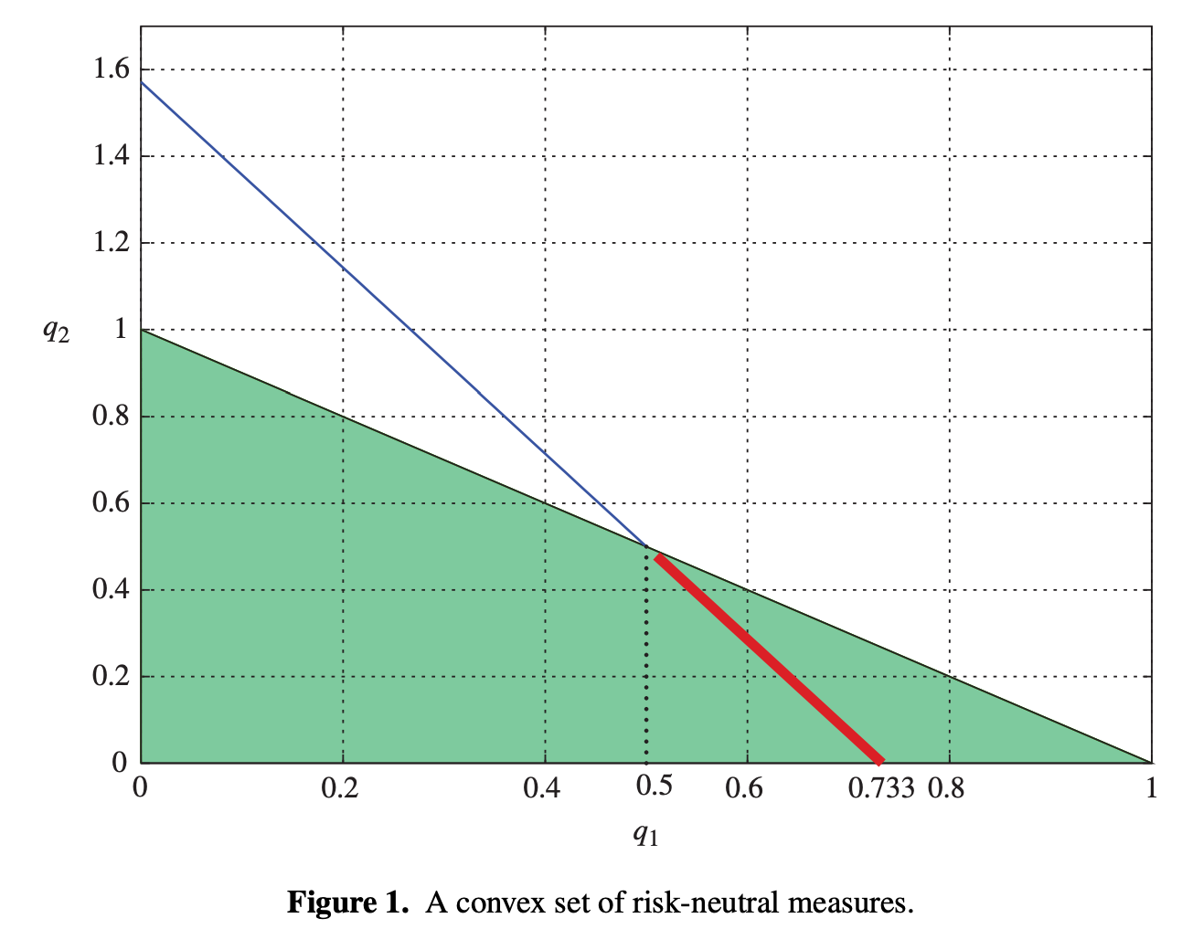
Since q1 + q2 ≤ 1, the shaded triangle represents all probability measures. The riskneutral probability measure must also satisfy $0.15q_1 + 0.07q_2 = 0.11$

The points on this line that are also inside the triangle, represent risk-neutral probability measures. $\rightarrow$ The solution to the market restriction equation is not unique, but is composed of the 1-dimensional convex polytope of solutions represented by the thick line segment in Figure 1.

This market is not complete: We have two non-redundant claims and three states. Another way to say this is that, although A and O are linearly independent, they do not form a basis for $\mathbb{R}^3$
.

Therefore one cannot arrange any conceivable payoff vector using only A and O.