1. Structure of generic bayesian inference procedure
- Design a proper prior : prior design is important for scientific applications, and various types of prior is used in different cases
- Non-informative prior, Spike-and-slab prior, ...
- Likelihood term , i.e. data generating mechanism takes account into contribution of dataset(observations)
- Posterior can be obtained in a closed form for some prior designs(conjugate priors), while most of the case we only can calculate 'kernel' of the distribution since , and integral of the nominator is usually hard to calculate.
- Perform some statistical inferences on posterior distribution, for example calculate the posterior mean or credible interval.
2. Bayesian inference on posterior distribution
- Posterior mean: (monte carlo estimate)
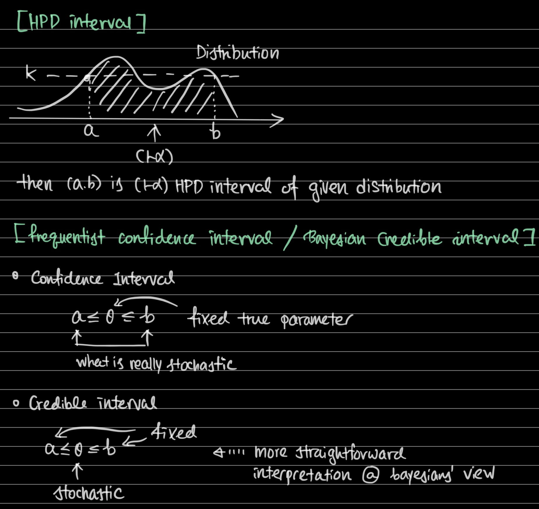
- Bayesian credible interval: credible interval (a,b) for a,b, s.t.
- HPD interval(highest posterior density interval) and its interpretation
3. Choosing priors
- If data size n increases, posterior becomes close to likelihood
- For large n, MLE ~ posterior mode(mean)
- Thus point estimate and uncertainty becomes close in bayesian & frequentist's view.
- But not always n is sufficiently large & similarity assumption requires some regularity conditions to be met.
- Prior does matter, and cause different result compared with MLE approach in bayesian inference.
- Several ways to choose priors
- Non-informative priors (e.g. Uniform distribution) : Same density across different parameter space
- When we don't have any pre-knowledge
- Bayesian inference & MLE will be similar
- Posterior mode = Maximum likelihood estimate when prior is non-informative
- Convenient priors(i.e. conjugate priors) : Analytically closed-form posteriors are preferred
- By choosing proper priors we can make posterior in a form of beta, normal, inverse-gamma distributions.
- Easy to calculate mean & credible interval
- Select conjugate priors
- Expert opinion : Realistic range of parameters exists(e.g. decay rate ), pre-knowledge can be adopted
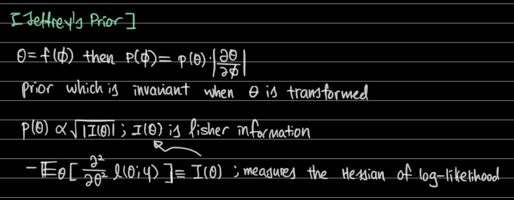
- Rule-based priors(e.g. Jeffrey's prior)
- Non-informative priors (e.g. Uniform distribution) : Same density across different parameter space
4. Conjugate priors
- Not always posterior is tractable in closed form, but special pairs of (prior, likelihood) can lead to tractable posterior
- Pairs of conjugate prior and likelihood
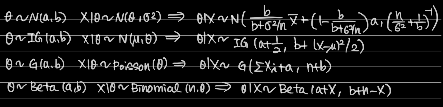
- BE CAREFUL!
- IG(a,b): shape and rate parameter
- G(a,b): shape and rate parameter
- Mean of G(a,b) = ab: for shape and scale parameter
- Mean of IG(a,b) = b/(a-1): for shape and scale parameter
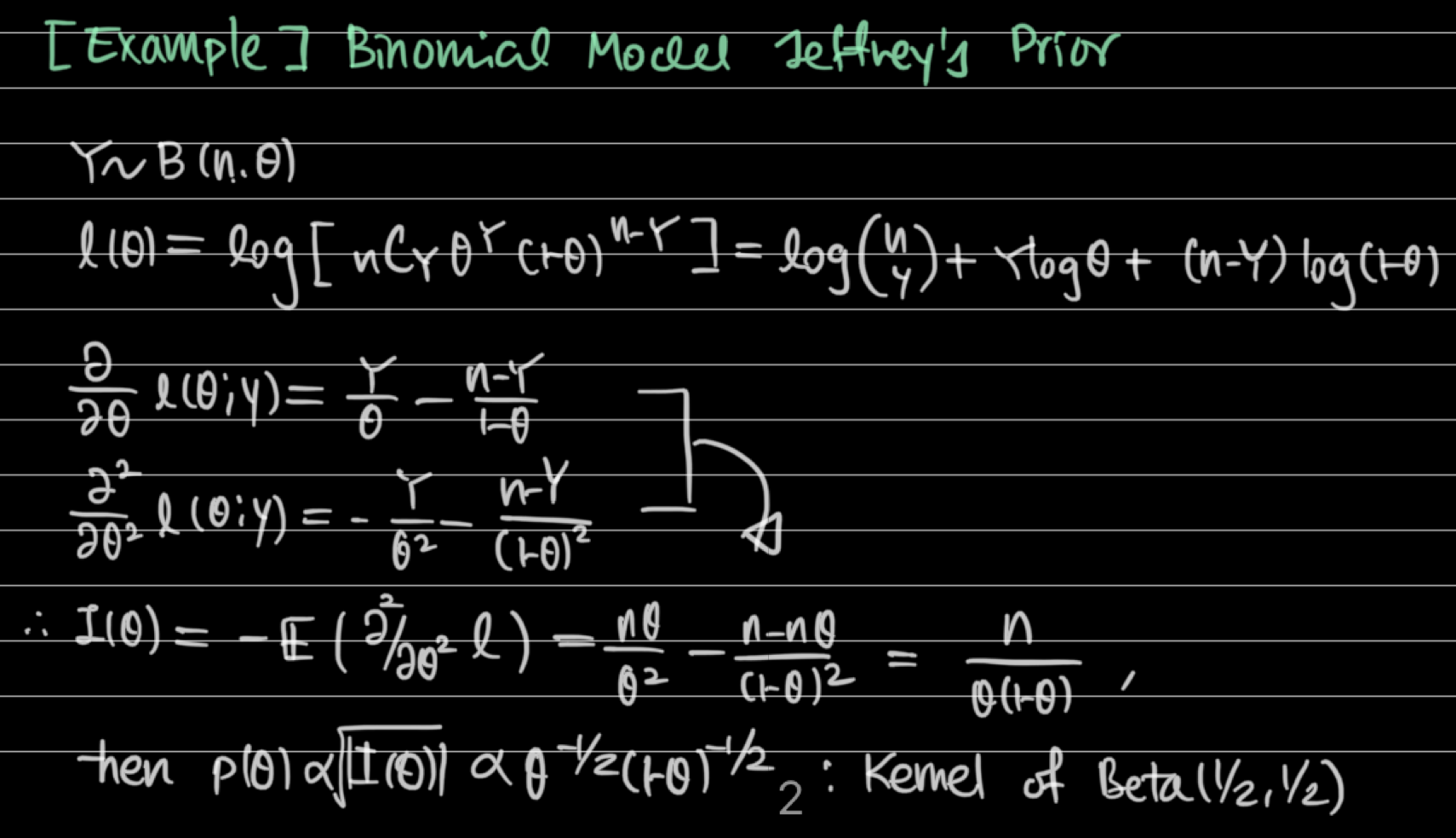
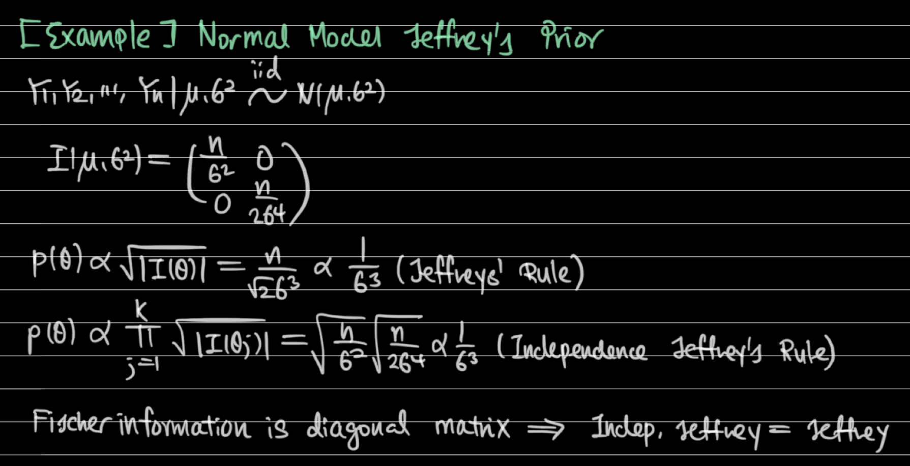
5. Jeffrey prior
- Prior which is invariant to transformations
5. Non-conjugate families
- Gibbs sampler
- Draw samples from full conditional of posterior distribution
- Metropolis-hastings algorithm
- Draw samples even if we don't know the full conditional of posterior distribution

interested in 🖥️,🧠,🧬,⚛️