타이타닉 머신러닝(1)

이젠 내가 아니라 컴퓨터가 일 할 차례이다. 여러 머신러닝 모델에 방금 가공한 데이터를 넣고 정확도를 측정해보자.

from sklearn.linear_model import LogisticRegression
from sklearn import svm #Support Vector Machine
from sklearn.ensemble import RandomForestClassifier
from sklearn.neighbors import KNeighborsClassifier
from sklearn.naive_bayes import GaussianNB
from sklearn.tree import DecisionTreeClassifier
from sklearn.model_selection import train_test_split
from sklearn import metrics
from sklearn.metrics import confusion_matrix

train데이터와 test데이터를 구분해 넣어준다.

train,test=train_test_split(train,test_size=0.3,random_state=0,stratify=train['Survived'])
train_X=train[train.columns[1:]]
train_Y=train[train.columns[:1]]
test_X=test[test.columns[1:]]
test_Y=test[test.columns[:1]]
X=train[train.columns[1:]]
Y=train['Survived']

model=svm.SVC(kernel='rbf',C=1,gamma=0.1)
model.fit(train_X,train_Y)
prediction1=model.predict(test_X)
print('Accuracy of rbf SVM is ',metrics.accuracy_score(prediction1,test_Y))

Radial Support Vector Machines(rbf-SVM)는 약 83%의 정확도가 나온다. 헌데 경고창이 떠서 알아보니,Scikit-learn 모델은 타겟 변수를 1차원 배열로 받기 때문에 이러한 경고가 발생한다고 한다. 우리가 준 데이터가 column-vector(열 벡터) 형태의 배열을 가지고 있었기에 이런 경고가 발생했고, 모델의 성능에 직접적 영향은 없다지만 영 찝찝하다.
맨 위 라이브러리를 가져오는 코드에

train_Y = np.ravel(train_Y)
test_Y = np.ravel(test_Y)

을 추가해 해결해주자.

다음은 Linear Support Vector Machine(linear-SVM)

model=svm.SVC(kernel='linear',C=0.1,gamma=0.1)
model.fit(train_X,train_Y)
prediction2=model.predict(test_X)
print('Accuracy of Linear SVM is ',metrics.accuracy_score(prediction2,test_Y))

다음은 Logistic Regression

model=LogisticRegression()
model.fit(train_X,train_Y)
prediction3=model.predict(test_X)
print('Accuracy of the LogisticRegression is ',metrics.accuracy_score(prediction3,test_Y))

다음은 Decision Tree

model=DecisionTreeClassifier()
model.fit(train_X,train_Y)
prediction4=model.predict(test_X)
print('Accuracy of the Decision Tree is ',metrics.accuracy_score(prediction4,test_Y))

다음은 K-Nearest Neighbours(KNN)

model=KNeighborsClassifier() 
model.fit(train_X,train_Y)
prediction5=model.predict(test_X)
print('Accuracy of the KNN is ',metrics.accuracy_score(prediction4,test_Y))

KNN은 n_neighbours attribute값에 따라 정확도가 달라진다고 한다. 값을 바꿈에 따라 정확도가 어떻게 변화는지 보고, 최적의 값을 확인해보자.

a_index = list(range(1, 11))
a = []  # 빈 리스트로 초기화

for i in range(1, 11):
    model = KNeighborsClassifier(n_neighbors=i)
    model.fit(train_X, train_Y)
    prediction = model.predict(test_X)
    accuracy = metrics.accuracy_score(prediction, test_Y)
    a.append(accuracy)  # 정확도를 리스트에 추가

# 리스트를 Pandas Series로 변환
a = pd.Series(a, index=a_index)

plt.plot(a_index, a)
plt.xticks(a_index)
fig = plt.gcf()
fig.set_size_inches(12, 6)
plt.show()

print('Accuracy of different values of n are:', a.values, 'with the max value as', a.values.max())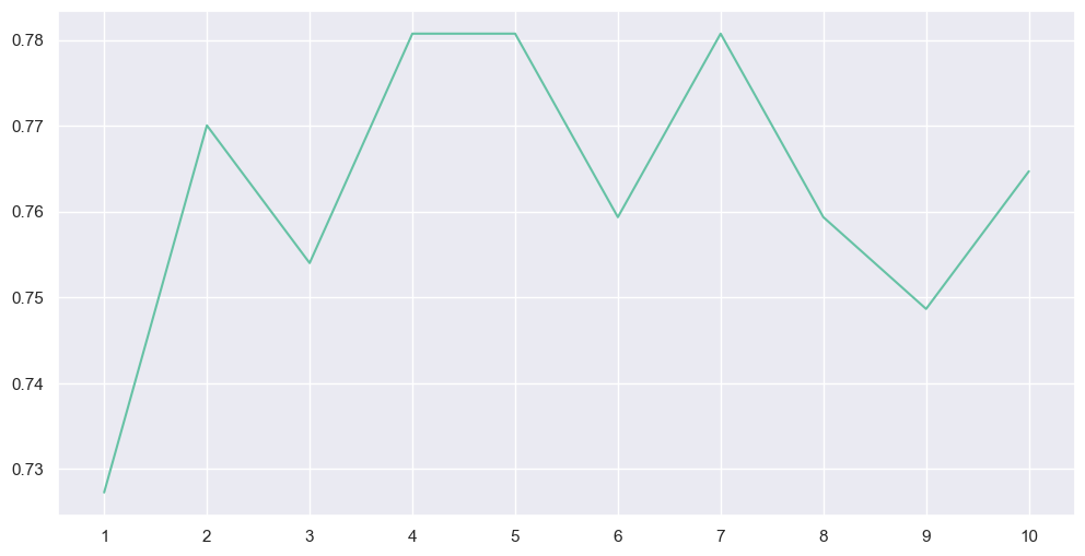

n_neighbours attribute값이 4,5,7일 때 가장 정확도가 높음을 확인할 수 있다.

다음은 Gaussian Naive Bayes 이다.

model=GaussianNB()
model.fit(train_X,train_Y)
prediction6=model.predict(test_X)
print('Accuracy of the NaiveBayes is ',metrics.accuracy_score(prediction6,test_Y))

다음은 Random Forest 이다.

model=RandomForestClassifier(n_estimators=100)
model.fit(train_X,train_Y)
prediction7=model.predict(test_X)
print('Accuracy of the Random Forest is ',metrics.accuracy_score(prediction7,test_Y))

이제 K-Fold Cross Validation 교차 검증을 통해 각 모델의 평균 정확도와 표준편차를 비교해보자. n_neighbours attribute값에는 방금 가장 정확도가 높았던 7을 넣었다.

from sklearn.model_selection import KFold
from sklearn.model_selection import cross_val_score
from sklearn.model_selection import cross_val_predict
kfold = KFold(n_splits=10,shuffle=True, random_state=22)
xyz = []
accuracy = []
std = []
classifiers=['Linear Svm','Radial Svm','Logistic Regression','KNN','Decision Tree','Naive Bayes','Random Forest']
models=[svm.SVC(kernel='linear'),svm.SVC(kernel='rbf'),LogisticRegression(),KNeighborsClassifier(n_neighbors=7),DecisionTreeClassifier(),GaussianNB(),RandomForestClassifier(n_estimators=10)]
for i in models:
    model = i
    cv_result = cross_val_score(model,X,Y,cv=kfold,scoring="accuracy")
    cv_result=cv_result
    xyz.append(cv_result.mean())
    std.append(cv_result.std())
    accuracy.append(cv_result)
new_models_dataframe2=pd.DataFrame({'CV Mean':xyz,'Std':std},index=classifiers)
new_models_dataframe2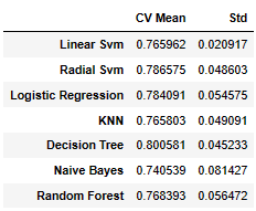

평균 정확도는 Decision Tree가 가장 높고, 표준편차는 Linear Svm이 가장 낮았다. 이를 시각화 하면 다음과 같다.

plt.subplots(figsize=(12,6))
box=pd.DataFrame(accuracy,index=[classifiers])
box.T.boxplot()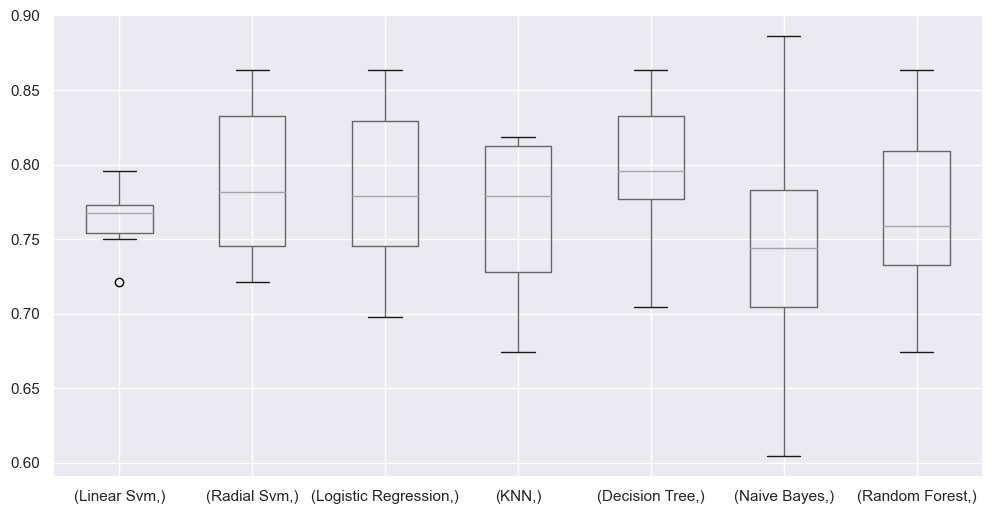

이렇게 모델의 특성을 비교하면 프로젝트 목표에 따라 알맞은 모델을 선정하는데 큰 도움이 될 것이다.

다음은 Confusion Matrix로 Classifier에 의해 만들어지는 많은 정확한/부정확한 classification을 만들어준다.

f,ax=plt.subplots(3,3,figsize=(12,10))
y_pred=cross_val_predict(svm.SVC(kernel='rbf'),X,Y,cv=10)
sns.heatmap(confusion_matrix(Y,y_pred),ax=ax[0,0],annot=True,fmt='2.0f')
ax[0,0].set_title('Matrix for rbf-SVM')
y_pred=cross_val_predict(svm.SVC(kernel='linear'),X,Y,cv=10)
sns.heatmap(confusion_matrix(Y,y_pred),ax=ax[0,1],annot=True,fmt='2.0f')
ax[0,1].set_title('Matrix for Linear-SVM')
y_pred=cross_val_predict(KNeighborsClassifier(n_neighbors=9),X,Y,cv=10)
sns.heatmap(confusion_matrix(Y,y_pred),ax=ax[0,2],annot=True,fmt='2.0f')
ax[0,2].set_title('Matrix for KNN')
y_pred=cross_val_predict(RandomForestClassifier(n_estimators=100),X,Y,cv=10)
sns.heatmap(confusion_matrix(Y,y_pred),ax=ax[1,0],annot=True,fmt='2.0f')
ax[1,0].set_title('Matrix for Random-Forests')
y_pred=cross_val_predict(LogisticRegression(),X,Y,cv=10)
sns.heatmap(confusion_matrix(Y,y_pred),ax=ax[1,1],annot=True,fmt='2.0f')
ax[1,1].set_title('Matrix for Logistic Regression')
y_pred=cross_val_predict(DecisionTreeClassifier(),X,Y,cv=10)
sns.heatmap(confusion_matrix(Y,y_pred),ax=ax[1,2],annot=True,fmt='2.0f')
ax[1,2].set_title('Matrix for Decision Tree')
y_pred=cross_val_predict(GaussianNB(),X,Y,cv=10)
sns.heatmap(confusion_matrix(Y,y_pred),ax=ax[2,0],annot=True,fmt='2.0f')
ax[2,0].set_title('Matrix for Naive Bayes')
plt.subplots_adjust(hspace=0.2,wspace=0.2)
plt.show()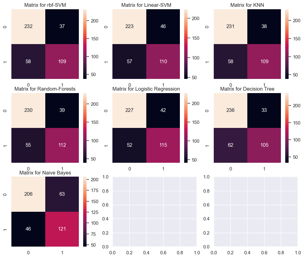

위 사각형에서 0은 사망,1은 생존이다. 0/0과 1/1 은 제대로 예측한 것이고, 0/1,1/0은 잘못 예측한 것이다. 즉 이 그래프를 통해 같은 정확도라도 이 모델이 생존자를 잘 찾는 모델인지, 사망자를 잘 찾는 모델인지를 알 수있는 부분이다. 타이타닉 예제에는 생존/사망 2가지 경우 뿐이라 의미없어 보일지라도, ComputerVision 부분에서는 여러 객체를 동시에 탐지하는 경우가 많아 특정 객체를 잘 잡는 모델을 찾는데 도움이 많이 된다. 프로젝트 목표가 여러 과일 중 사과를 골라내는 것이라면, 다른 과일에 대한 정확도가 떨어지더라도 사과에 대한 정확도만 높다면 그 모델은 채용 가치가 생긴다는 것이다.

다음은 Hyper-Parameters Tuning으로 parameter를 바꿔가며 최적의 값을 찾는 것이다. 예시로 SVM에서 C와 gamma값을 변경시켜 감에 따라 결과를 확인하자.

from sklearn.model_selection import GridSearchCV
C=[0.05,0.1,0.2,0.3,0.25,0.4,0.5,0.6,0.7,0.8,0.9,1]
gamma=[0.1,0.2,0.3,0.4,0.5,0.6,0.7,0.8,0.9,1.0]
kernel=['rbf','linear']
hyper={'kernel':kernel,'C':C,'gamma':gamma}
gd=GridSearchCV(estimator=svm.SVC(),param_grid=hyper,verbose=True)
gd.fit(X,Y)
print(gd.best_score_)
print(gd.best_estimator_)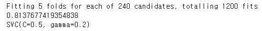

C=0.5, gamma=0.2일때 가장 결과가 좋다는 걸 볼 수 있다.

Random Forests를 예시로 하나 더 확인해보자.

n_estimators=range(100,1000,100)
hyper={'n_estimators':n_estimators}
gd=GridSearchCV(estimator=RandomForestClassifier(random_state=0),param_grid=hyper,verbose=True)
gd.fit(X,Y)
print(gd.best_score_)
print(gd.best_estimator_)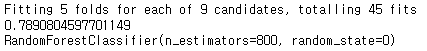

n_estimators값이 800일때 가장 좋음을 알 수 있다.