딥러닝-3단계(다차원, 추가 기능)

1. 차원

• 우리가 numpy를 통해 만들었던 array에 대해서 살펴보자.

  • image.shape을 했을 때, (1,)/(1,2)/(1,2,3)의 출력값을 본다면 순서대로 1차원, 2차원, 3차원이라고 생각한다. 이는 데이터 형태의 맥락에서 본 차원이다.```

  • df를 봤을 때, x축에 각각의 관측치가 3개 있고 y축에도 관측치가 3개가 있다. 그렇다면 (3,3)의 shape를 띄고 있을 텐데, 데이터 공간의 맥락에서 본다면 이는 9차원을 지닌다고 할 수 있다.

  • 즉, 관측치(독립적인)가 하나의 축을 만든다고 생각하면 이해가 쉽다.

실습 1.

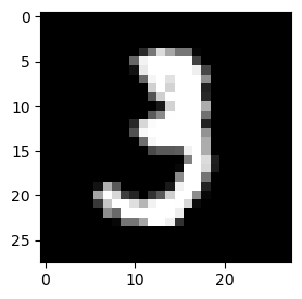
# 데이터 준비
(x_train, y_train), (x_test, y_test) = tf.keras.datasets.mnist.load_data()
print(x_train.shape, y_train.shape)
print(x_test.shape, y_test.shape)
<출력>
(60000, 28, 28) (60000,)
(10000, 28, 28) (10000,)
-> 데이터 형태 : 3차원이다.
-> 데이터 공간 : x, y 축 모두 28개의 관측치로 이뤄졌다. 즉, 784차원이다.

# 데이터 확인
print('정답 :', y_train[10])

plt.figure(figsize=(3,3))
plt.imshow(x_train[10], cmap='gray')       # 이미지 출력할 때 plt.imshow사용
plt.show()
<출력>
정답 : 3

---

2. 다 차원의 데이터 딥러닝 과정

• 다 차원의 관측치를 2차원의 df의 형태로 변환시킨다.
• y_train, y_test의 값에 대해서 one-hot 인코딩시킨다.

실습 2.

# 데이터를 준비한다
(x_train, y_train), (x_test, y_test) = tf.keras.datasets.fashion_mnist.load_data()

# 표로 만들기
x_train = x_train.reshape(60000, 784)
x_test = x_test.reshape(10000, 784)

# 원핫인코딩
y_train = pd.get_dummies(y_train)
y_test = pd. get_dummies(y_test)

print(x_train.shape, x_test.shape)
print(y_train.shape, y_test.shape)
<출력>
(60000, 784) (10000, 784)
(60000, 10) (10000, 10)

# 모델을 준비한다.
x = tf.keras.layers.Input(shape=[784])

h = tf.keras.layers.Dropout(0.6)(h)                
# 0.5이면 392개를 0으로 만들겠다임, 즉 방해하겠다는 거임. 왜? 성능이 너무 좋아서, 과적합을 방지하려고 하는 행위
h = tf.keras.layers.Dense(64, activation='swish')(h)
h = tf.keras.layers.BatchNormalization()(h)

h = tf.keras.layers.Dropout(0.5)(h)                
h = tf.keras.layers.Dense(32)(h)
h = tf.keras.layers.BatchNormalization()(h)        
# scale이 뒤죽박죽일 때 사용, 이상치가 많다면 standard를 별로 없다면 MinMax(Normalization)를 사용한다.
h = tf.keras.layers.Activation(activation = 'swish')(h)

# hidden에서는 특징을 간략하게 만드는 1) dropout 시키고 2) hidden layer 수 정하고 3) normalization하고 4) activation 하는게 더 좋다.

y = tf.keras.layers.Dense(10, activation= tf.keras.activations.softmax)(h)

model = tf.keras.Model(x, y)
model.compile(loss= categorical_crossentropy, metrics = accuracy)   

model.summary()

3. 기능(flatten, sparse_, model.fit(validation), 학습 과정 시각화)

• 1) flatten은 input에서 x의 shape=[784] 이렇게 사용했는데, shape=[28,28]이렇게 사용해도 알아서 펴주는 기능이다.
• 2) sparse_는 model.compile에서 loss와 metrics에서 추가로 입력해주며, 원핫인코딩을 알아서 해주는 기능이다.
  • 유의점은 y의 관측치가 아이리스의 '품명'이 아닌 number로 labeling 되어 있는 경우에만 사용할 수 있는 방법이다.
• 3) validation은 모델 학습과 같이 실행시키는데 학습 도중에 오버피팅을 모니터링 하는데 사용된다.
  • val_loss가 늘어나면 오버피팅이구나 판단한다.
  • val_loss가 떨어지면 학습되고 있구나 판단한다.
  • validation = 0.2이면, 60000개의 데이터에서 20%를 벨리데이션에 사용하고 남은 80%를 학습에 사용한다.

실습 3-1

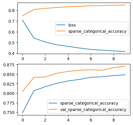
# 모델 준비

x = tf.keras.layers.Input(shape=[28, 28])
h = tf.keras.layers.Flatten()(x)

h = tf.keras.layers.Dropout(0.5)(h)
h = tf.keras.layers.Dense(128, activation = tf.keras.activations.swish)(h)
h = tf.keras.layers.BatchNormalization()(h)

y = tf.keras.layers.Dense(10, activation= tf.keras.activations.softmax)(h)

model = tf.keras.Model(x, y)
model.compile(loss= tf.keras.losses.sparse_categorical_crossentropy, metrics = tf.keras.metrics.sparse_categorical_accuracy)   

# 풀어서 activation, loss와 metrics 작성해주면 다른 방법들이 어떤게 있는지 확인하면서 사용할 수 있음. 공부에 도움이 됨. 그냥 작성해줘도 됨.

model.summary()
<출력>
Model: "model_9"
_________________________________________________________________
 Layer (type)                Output Shape              Param #   
=================================================================
 input_10 (InputLayer)       [(None, 28, 28)]          0         
                                                                
 flatten_9 (Flatten)         (None, 784)               0         
                                                               
 dropout_14 (Dropout)        (None, 784)               0         
                                                              
 dense_23 (Dense)            (None, 128)               100480    
                                                             
 batch_normalization_14 (Ba  (None, 128)               512       
 tchNormalization)                                               
                                                            
 dense_24 (Dense)            (None, 10)                1290      
                                                           
=================================================================
Total params: 102282 (399.54 KB)
Trainable params: 102026 (398.54 KB)
Non-trainable params: 256 (1.00 KB)
_________________________________________________________________

# 모델 학습
result = model.fit(x_train, y_train, epochs=10, batch_size = 300, validation_split=0.2)
<출력>
Epoch 10/10
192/192 [==============================] - 3s 13ms/step - loss: 0.6932 - accuracy: 0.7483 - val_loss: 0.4857 - val_accuracy: 0.8203

# 학습 과정 확인
reslut.history
입력하면 epoch 단계마다의 loss, accuracy, val_loss, val_accuracy를 확인할 수 있다.

# 학습 과정 시각화
plt.subplot(2,1,1)
plt.plot(result.history['loss'])
plt.plot(result.history['sparse_categorical_accuracy'])
plt.legend(['loss', 'sparse_categorical_accuracy'])

plt.subplot(2,1,2)
plt.plot(result.history['sparse_categorical_accuracy'])
plt.plot(result.history['val_sparse_categorical_accuracy'])
plt.legend(['sparse_categorical_accuracy', 'val_sparse_categorical_accuracy'])
<출력>

실습 3-2(validation, early stop)

• val_loss가 올라가면, 즉 과적합 발생 갯수가 특정 갯수에 도달했을 때, 학습을 자동으로 종료시키는 방법이다.

# 모델 준비

x = tf.keras.layers.Input(shape=[32, 32, 3])
h = tf.keras.layers.Flatten()(x)

h = tf.keras.layers.Dropout(0.5)(h)
h = tf.keras.layers.Dense(24, activation = 'swish')(h)
h = tf.keras.layers.BatchNormalization()(h)

y = tf.keras.layers.Dense(10, activation='softmax')(h)

model = tf.keras.Model(x, y)
model.compile(loss='sparse_categorical_crossentropy', metrics = 'accuracy',
             optimizer = tf.keras.optimizers.Adam(learning_rate=0.0001))

model.summary()
<출력>
Model: "model_10"
_________________________________________________________________
 Layer (type)                Output Shape              Param #   
=================================================================
 input_11 (InputLayer)       [(None, 32, 32, 3)]       0         
                                                              
 flatten_10 (Flatten)        (None, 3072)              0         
                                                             
 dropout_15 (Dropout)        (None, 3072)              0         
                                                            
 dense_25 (Dense)            (None, 24)                73752     
                                                           
 batch_normalization_15 (Ba  (None, 24)                96        
 tchNormalization)                                               
                                                          
 dense_26 (Dense)            (None, 10)                250       
                                                         
=================================================================

# 모델 학습
early = tf.keras.callbacks.EarlyStopping(
    monitor = 'val_loss',        # 디폴트 값이라 안넣어줘도 됨.
    min_delta=0,                 # 얘도 디폴트 값임.
    patience=10,                 # 이 횟수 동안 개선이 없으면 끝냄.
    restore_best_weights=True,   # False - > 맨 마지막 학습된 상태로 출력하겠다.  True -> val_loss가 낮았던 모델로 출력하겠다.
)

model.fit(x_train, y_train, epochs=150, 
          batch_size=512, validation_split=0.2, callbacks=[early])
<출력>
쭈르륵 학습 되다가 val_loss가 올라가는 횟수가 10번이 될 때, 학습을 자동으로 멈춘다.

실습 4(skip connection)

• hidden layer에 add를 for 구문을 통해서 깊은 망 신경학습을 하는 방법이다.

# 모델 준비

x = tf.keras.layers.Input(shape=[32, 32, 3])
h = tf.keras.layers.Flatten()(x)

h = tf.keras.layers.Dropout(0.5)(h)
h = tf.keras.layers.Dense(128)(h)
h = tf.keras.layers.BatchNormalization()(h)
h = tf.keras.layers.Activation('swish')(h)

for i in range(32):
    h1 = tf.keras.layers.Dropout(0.5)(h)
    h1 = tf.keras.layers.Dense(128)(h)
    h1 = tf.keras.layers.BatchNormalization()(h1)
    h = tf.keras.layers.Add()([h, h1])
    h = tf.keras.layers.Activation('swish')(h)

y = tf.keras.layers.Dense(10, activation='softmax')(h)

model = tf.keras.Model(x, y)
model.compile(loss='sparse_categorical_crossentropy', metrics = 'accuracy',
             optimizer = tf.keras.optimizers.Adam(learning_rate=0.0001))        #optimizers.SGD(learning_rate=0.001)

model.summary()
<출력>
32번의 깊은 망 신경 학습을 하게 된다.

# 모델 학습
early = tf.keras.callbacks.EarlyStopping(patience=10, restore_best_weights=True)

model.fit(x_train, y_train, epochs=150, 
          batch_size=512, validation_split=0.2, callbacks=[early])

<출력>
Epoch 24/150
79/79 [==============================] - 10s 128ms/step - loss: 1.9701 - accuracy: 0.2805 - val_loss: 1.9204 - val_accuracy: 0.3002