딥러닝-2단계(함수, hidden layer, 입력값)

엔지니어 큐브·2023년 9월 5일

딥러닝

목록 보기

2/5

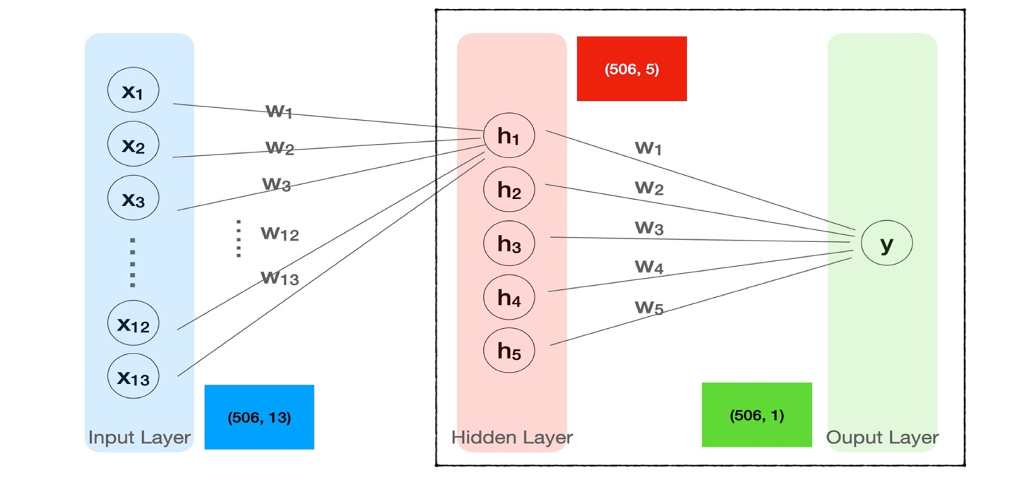
1) hidden layer

피처들의 특성을 더 잘 분화시키기 위하여 사용하며 입력값(x) 다음에 위치한다.

h = tf.keras.layers.Dense(64, activation='swish')(x) 위와 같은 형태로 작성한다.

activation = 의 값은 'swish' or 'GELU'의 활성화 함수를 최근 많이 사용한다.

히든의 차원 수는 입력(x)의 차원 수 보다 많아도 상관없다. 보통 2의 배수로 놓는다.

hidden layer는 여러개 들어가도 된다.

실습 1

df = pd.read_csv(path)
target = 'medv'
독립 = df.drop(target, axis =1)
종속 = df.loc[:,target]

x = tf.keras.layers.Input(shape=[13])
h = tf.keras.layers.Dense(64, activation = 'swish')(x)
h = tf.keras.layers.Dense(64, activation = 'swish')(h)
y = tf.keras.layers.Dense(1)(h)
model = tf.keras.Models(x, y)
model.compile(loss='mse')

model.summary()
<출력>
Model: "model_2"
_________________________________________________________________
 Layer (type)                Output Shape              Param #   
=================================================================
 input_3 (InputLayer)        [(None, 13)]              0         
                                                                
 dense_5 (Dense)             (None, 64)                896       #(13+1)*64 = 896
                                                                
 dense_6 (Dense)             (None, 64)                4160      #(64+1)*64 = 4160
                                                                
 dense_7 (Dense)             (None, 1)                 65        #(64+1) = 65
                                                                
=================================================================
Total params: 5121 (20.00 KB)

2) loss를 0으로 낮추는 방법

hidden layer와 epoches = high를 통한 방법은 모델 fit 횟수를 많이 함으로써 loss를 줄이는 방법이다.

hidden layer를 작성하고, 그 다음에 BachNormalization을 추가 입력하는 방법이 있다.

많이 사용하는 방법이고 거의 항상 적용한다.

h = tf.keras.layers.BatchNormalization()(h)

bach_size를 설정해주는 방법이 있다.

1) bach_size를 지정하지 않으면, 디폴트는 32이고 만약 150개의 피처가 있다면 5 배치만 형성된다. 출력에서 epoche 아래에 있는 숫자가 bach를 의미한다.

2) model.fit(x, y, epochs=20)을 실행시키면 돌아가는 출력 값에서 몇 배치가 형성됐는지 확인할 수 있다.

3) bach_size가 낮다면 랜덤으로 배치가 형성되기 때문에, 잘못된 군집으로 인해 회귀선의 기울기가 많이 흔들리면서, loss 값이 흔들리게 된다.

4) bach_size를 크게 설정하면, 군집이 비슷한 양상으로 잡히기 때문에, loss 값이 흔들리는 현상이 줄어든다. 하지만 적절한 size를 잡아야한다.

5) 만약 피처가 적다면, bach_size=피처값 으로 잡아주면 좋다.

optimizer = 값을 지정해준다.

model.compile(loss='mse', optimizer = 'adam')의 방식으로 작성한다.

실습 2

# 데이터 준비
df = pd.read_csv(path)
target =['품종']
x = df.drop(target, axis=1)
y = df.loc[:, target]

#모델 준비
x_train = tf.keras.layers.Input(shape=[4])

h = tf.keras.layers.Dense(64, activation='swish')(x_train)               
h = tf.keras.layers.BatchNormalization()(h)

h = tf.keras.layers.Dense(64, activation='swish')(h)
h = tf.keras.layers.BatchNormalization()(h)

y_train = tf.keras.layers.Dense(3, activation='softmax')(h)

model = tf.keras.Model(x_train, y_train)
model.compile(loss = 'categorical_crossentropy', metrics = 'accuracy')

model.summary()
<출력>
_________________________________________________________________
 Layer (type)                Output Shape              Param #   
=================================================================
 input_8 (InputLayer)        [(None, 4)]               0         
                                                              
 dense_12 (Dense)            (None, 64)                320       
                                                               
 batch_normalization (Batch  (None, 64)                256       
 Normalization)                                                  
                                                              
 dense_13 (Dense)            (None, 64)                4160      
                                                             
 batch_normalization_1 (Bat  (None, 64)                256       
 chNormalization)                                                
                                                              
 dense_14 (Dense)            (None, 3)                 195       
                                                                
=================================================================

# 모델 fitting
model.fit(x, y, epochs=500, verbose=0, batch_size = 150)                   
model.fit(x, y, epochs=20, batch_size = 150)        

<출력>(마지막 반복만 가져왔음)
Epoch 20/20
1/1 [==============================] - 0s 10ms/step - loss: 8.6399e-05 - accuracy: 1.0000

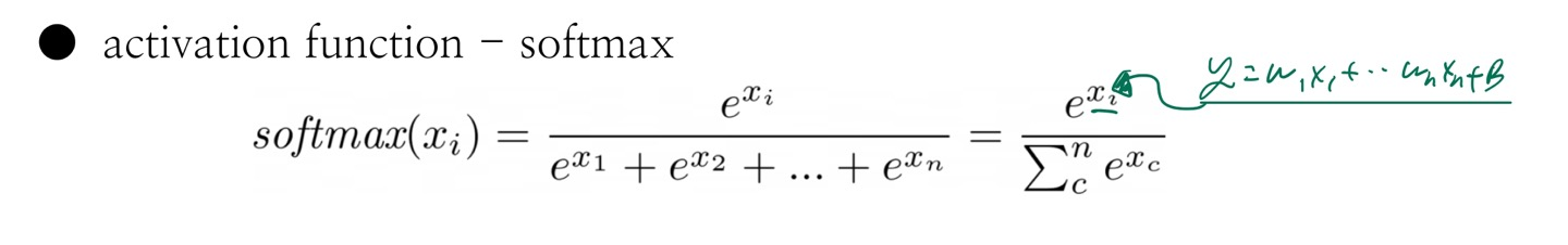
3) softmax

y1 = softmax(w1x1 + w2x2 ... + w_n x_n + b)

y2 = softmax(w1x1 + w2x2 ... + w_n x_n + b)

y3 = softmax(w1x1 + w2x2 ... + w_n x_n + b)

이러한 각 칼럼에 대한 회귀식이 softmax에 입력되고, 출력되는 ey1+ey2+ey3 = 1이 나온다.

실습 3

# 아이리스 문제사용, 모델 만드는 과정 생략.
--------------------------------------------------------------------
# 가중치와 편향 값 확인
model.get_weights()
<출력>
[array([[ 0.87844133,  0.7547402 ,  0.16198924],
        [ 1.1496656 , -0.31766355, -0.55518866],
        [-1.3137527 , -0.15838438,  0.2865614 ],
        [-2.1435575 ,  0.47845492,  2.4735708 ]], dtype=float32),
 array([ 0.67414737,  0.4880521 , -0.4638665 ], dtype=float32)]
--------------------------------------------------------------------
# 입력 값 확인
x_train[:5]
<출력>
	꽃잎길이	꽃잎폭	 꽃받침길이	꽃받침폭
0	5.1			3.5		1.4		0.2
1	4.9			3.0		1.4		0.2      <- softmax에 사용했음
2	4.7			3.2		1.3		0.2
--------------------------------------------------------------------
# 모델 예측 값 확인 (1)
model.predict(x_train[:5]).round(2)[1]
<출력>
0.9302478176181254 0.06848585038494003 0.0012663319969345747
--------------------------------------------------------------------
# softmax 함수에 식을 만들어서 모델 예측 값 확인 (2)
x1, x2, x3, x4 = 4.9, 3.0, 1.4, 0.2


y1 = 0.87844133*x1 + 1.1496656*x2 + -1.3137527*x3 + -2.1435575*x4 + 0.67414737
y2 = 0.7547402*x1 + -0.31766355*x2 + 0.15838438*x3 + 0.47845492*x4 + 0.4880521 
y3 = 0.16198924*x1 + -0.55518866*x2 + 0.2865614*x3 + 2.4735708*x4 + -0.4638665

ey1 = math.e ** y1
ey2 = math.e ** y2
ey3 = math.e ** y3

# softmax의 계산법임.
py1 = ey1/(ey1+ey2+ey3)
py2 = ey2/(ey1+ey2+ey3)
py3 = ey3/(ey1+ey2+ey3)

print(py1, py2, py3)
<출력>
softmax 예측 값 : 0.9302478176181254 0.06848585038494003 0.0012663319969345747

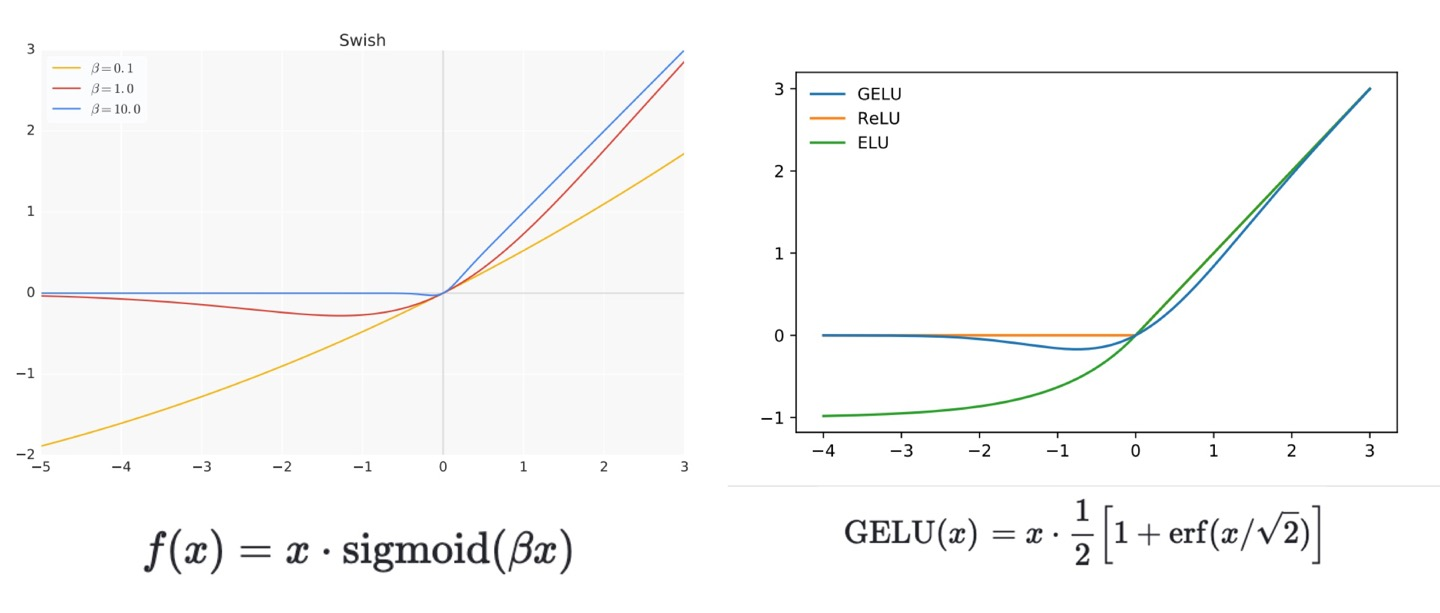
4) 활성화 함수

최근 사용되는 활성화 함수의 특징

미분 값이 1 보다 작으면 반복 fitting에 의한 중첩되어 미분값이 0으로 수렴해짐으로써, weight의 변화가 loss에 영향을 주지 못하는 결과를 극복함.

ReLU의 경우 미분점이 없었는데, 미분 가능한 지점을 형성하여 해당 문제를 극복함.

swish // GELU가 현재 좋은 활성화 함수이다.

5) optimizer

loss를 줄이기 위해 사용된다.

model.compile() 이 안에 작성해주면 된다. 아마 'adam'이 디폴트 값인 것으로 알고있다. 확실치는 않다.
x = tf.keras.Input(shape=[13])        
h = tf.keras.layers.Dense(64, activation='swish')(x)                
y = tf.keras.layers.Dense(1)(h)                     

model = tf.keras.Model(x, y)
model.compile(loss='mse', optimizer = 'adam')
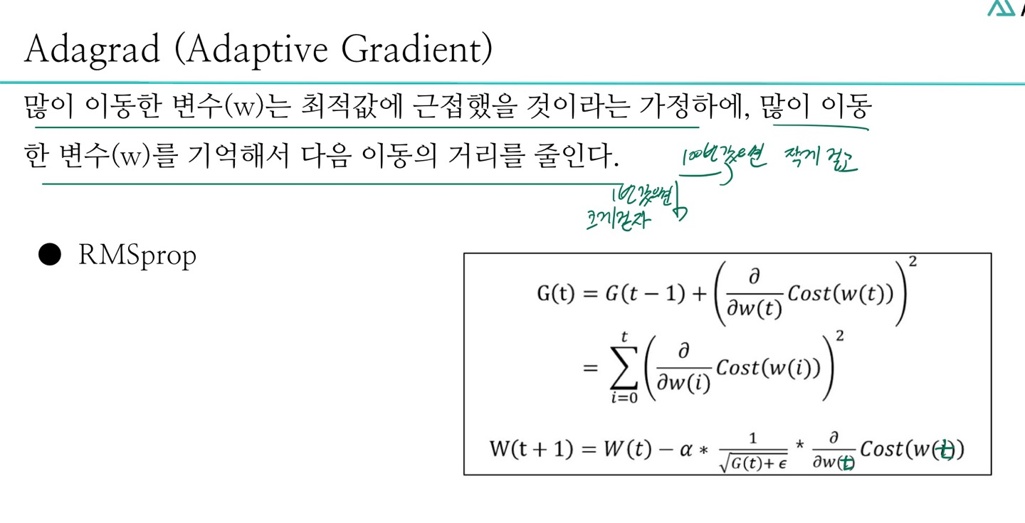
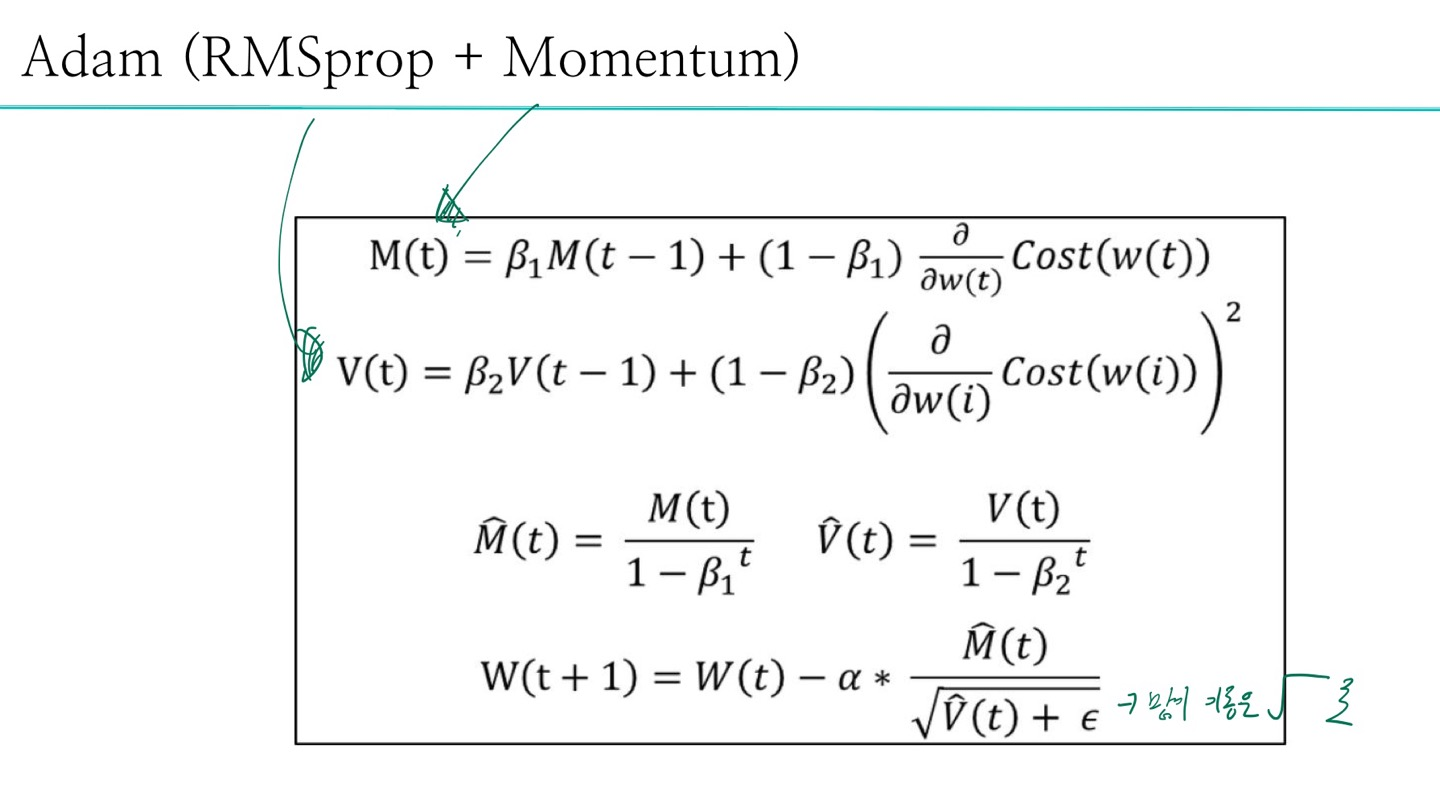
'adam', 'Adagrad' 두 가지의 입력값이 있다. 'adam'을 많이쓴다.

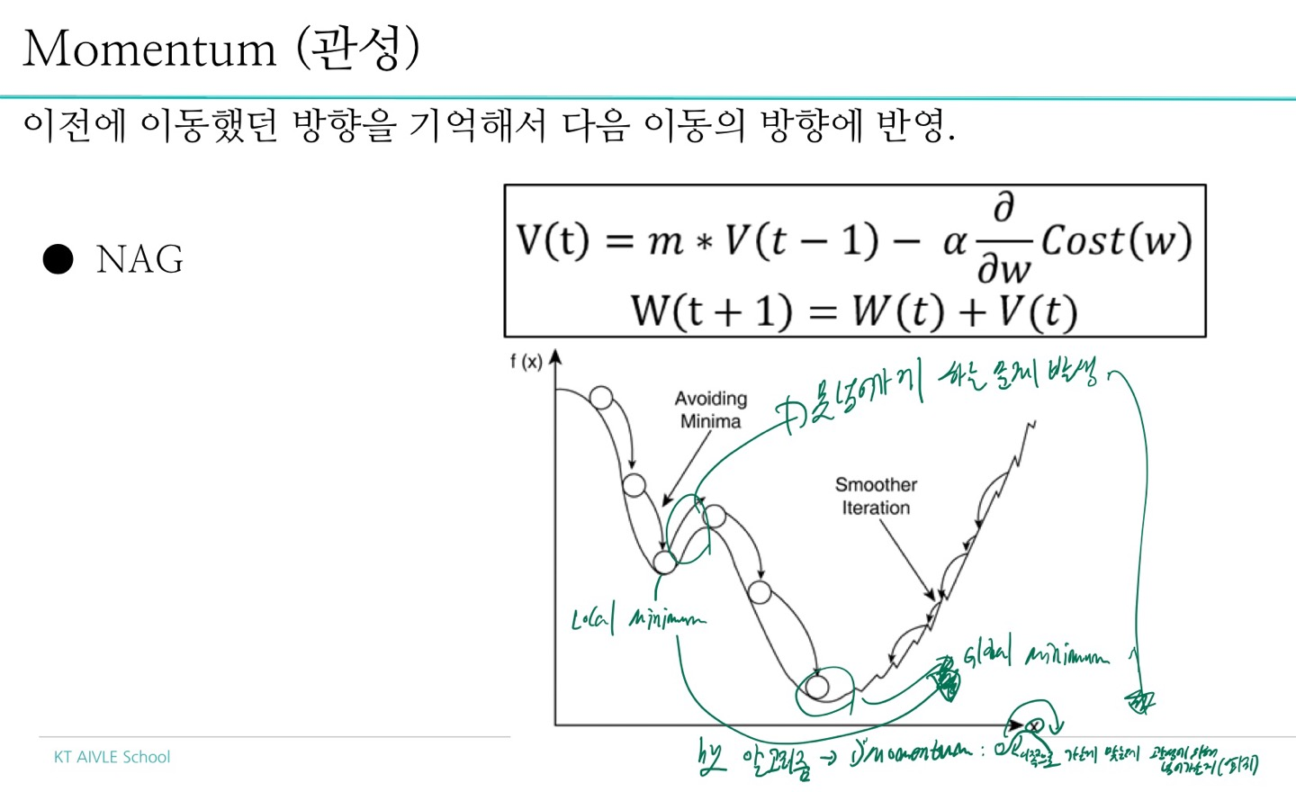
5-1) 개념

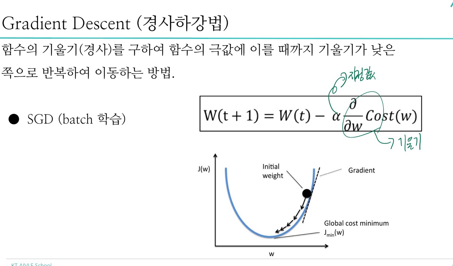
경사하강법

momentum

Adagrad

Adam

6) fit 함수의 동작 열어보기(GradientTape())

loss = tf.keras.losses.MeanSquaredError()
optim = tf.keras.optimizers.Adam(learning_rate=0.001)

for e in range(1000):
    with tf.GradientTape() as tape:                              # 미분
        pred = model(x_train.values, training=True)
        cost = loss(y_train.values, pred)             
        # cost : loss임, 종속.values는 정답 그리고 pred는 예측임 즉 cost는 오차값이라서 loss임
  
    grad = tape.gradient(cost, model.trainable_weights)
    optim.apply_gradients(zip(grad, model.trainable_weights))   # grad는 미분값 // trainalbe_은 w,b 값임.
    # grad랑 optim.apply~는 가중치 조절코드인데 이 2개를 통해서 cost를 작게 만들어야 한다.
    print(e, cost)      

<출력>(마지막꺼)
999 tf.Tensor(28.237234, shape=(), dtype=float32)        # error = 5