📊 원본 이미지로 분류

📌 이미지 분류 실습

1. 라이브러리 Import

import numpy as np
import matplotlib.pyplot as plt
from keras.datasets.mnist import load_data
from sklearn.preprocessing import MinMaxScaler
from keras.utils import to_categorical
from sklearn.model_selection import train_test_split
from keras.models import Model
from keras.layers import Input, Dense, Dropout, Flatten
from keras.optimizers import Adam
from sklearn.metrics import accuracy_score, roc_curve, auc

---

2. 데이터 준비

(x_train, y_train), (x_test, y_test) = load_data()
print(x_train.shape, y_train.shape, x_test.shape, y_test.shape)
# (60000, 28, 28) (60000,) (10000, 28, 28) (10000,)

---

3. 데이터 확인

print(x_train[0])
print(y_train[0])

---

4. 데이터 시각화

plt.imshow(x_train[0])
plt.show()

---

5. 데이터 차원 축소

x_train = x_train.reshape(-1, 784).astype('float32')
x_test = x_test.reshape(-1, 784).astype('float32')
print(x_train.shape, x_test.shape)
# (60000, 784) (10000, 784)

---

6. feature 정규화

scaler = MinMaxScaler()
x_train = scaler.fit_transform(x_train)
x_test = scaler.fit_transform(x_test)

---

7. label 원-핫 인코딩

y_train = to_categorical(y_train)
y_test = to_categorical(y_test)
print(y_train[0])
# [0. 0. 0. 0. 0. 1. 0. 0. 0. 0.]

---

8. 학습, 검증 데이터 분리

x_train, x_valid, y_train, y_valid = train_test_split(x_train, y_train, test_size=0.4, stratify=y_train, random_state=1)
print(x_train.shape, x_valid.shape, y_train.shape, y_valid.shape)
# (36000, 784) (24000, 784) (36000, 10) (24000, 10)

---

9. Functional API 모델 구축
[ Dropout 층 ]
- 은닉층에서 전체 노드 중 일부만 동작하도록 지정하는 층
- 모델 과적합을 방지하기 위해 사용한다.

inputs = Input(shape=(784, ))
net1= Dense(units=128, activation='relu')(inputs)
# flatten = Flatten(input_shape=(28, 28))(net1)   # reshape을 하지 않은 데이터의 차원 축소를 위한 층
drop1 = Dropout(rate=0.2)(net1)   # 이전 Dense층의 노드(128개) 중에서 20%로만 동작하도록 지정
outputs = Dense(units=10, activation='softmax')(net1)

model = Model(inputs, outputs)

---

10. 모델 학습 최적화 설정

model.compile(optimizer=Adam(learning_rate=0.001), loss='categorical_crossentropy', metrics=['acc'])

---

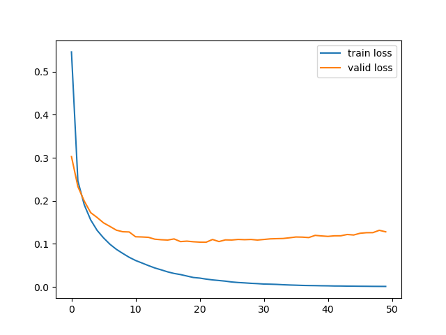
11. 모델 학습

history = model.fit(
    x=x_train,
    y=y_train,
    batch_size=256,
    epochs=50,
    validation_data=(x_valid, y_valid),
    verbose=0
)
plt.plot(history.history['loss'], label='train loss')
plt.plot(history.history['val_loss'], label='valid loss')
plt.legend()
plt.show()

---

12. 모델 검증

loss, acc = model.evaluate(
    x=x_test,
    y=y_test,
    batch_size=256,
    verbose=0
)
print('loss : ', loss)
print('acc : ', acc)
# loss :  0.11718954145908356
# acc :  0.9739999771118164

---

13. 모델 예측값, 실제값 비교

y_pred = model.predict(x_test)
y_pred = np.where(y_pred > 0.5, 1, 0)
print('예측값 : ', y_pred[:4])
print('실제값 : ', y_test[:4])
# 예측값 :  [[0 0 0 0 0 0 0 1 0 0]
#  [0 0 1 0 0 0 0 0 0 0]
#  [0 1 0 0 0 0 0 0 0 0]
#  [1 0 0 0 0 0 0 0 0 0]]
# 실제값 :  [[0. 0. 0. 0. 0. 0. 0. 1. 0. 0.]
#  [0. 0. 1. 0. 0. 0. 0. 0. 0. 0.]
#  [0. 1. 0. 0. 0. 0. 0. 0. 0. 0.]
#  [1. 0. 0. 0. 0. 0. 0. 0. 0. 0.]]

---

14. 분류모델 성능 평가 - 정확도

acc = accuracy_score(y_test, y_pred)
print('정확도 : ', acc)
# 정확도 :  0.9734

---

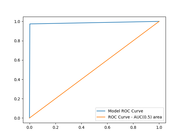
15. ROC 곡선 그리기

FPR, TPR, _ = roc_curve(y_test.flatten(), y_pred.flatten())
auc_value = auc(FPR, TPR)
plt.plot(FPR, TPR, label='Model ROC Curve')
plt.plot([0, 1], [0, 1], label='ROC Curve - AUC(0.5) area')
plt.legend()
plt.show()

---

16. AUC 면적값 추출

print('AUC 값 : ', auc_value)
# AUC 값 :  0.9852888888888889