📊 DL 다항분류

📌 다항분류란?

• 정의
  - 1개 이상의 독립변수로 레이블 내의 unique value 개수가 3개 이상인 레이블 중 하나로 분류하는 방법이다.

📌 DL 다항분류 실습

1. 라이브러리 Import

import pandas as pd
import numpy as np
import matplotlib.pyplot as plt
import seaborn as sns
from sklearn.preprocessing import LabelEncoder
from sklearn.model_selection import train_test_split
from keras.utils import to_categorical
from keras.models import Model
from keras.layers import Input, Dense
from keras.optimizers import Adam
from sklearn.metrics import accuracy_score, classification_report, roc_curve, auc

---

2. 데이터 준비

data = pd.read_csv('../testdata/iris.csv')
print(data.head())
print(data.shape)
#    Sepal.Length  Sepal.Width  Petal.Length  Petal.Width Species
# 0           5.1          3.5           1.4          0.2  setosa
# 1           4.9          3.0           1.4          0.2  setosa
# 2           4.7          3.2           1.3          0.2  setosa
# 3           4.6          3.1           1.5          0.2  setosa
# 4           5.0          3.6           1.4          0.2  setosa
# (150, 5)

---

3. 레이블 인코딩

encoder = LabelEncoder()
data['Species'] = encoder.fit_transform(data['Species'])
print(data['Species'].unique())
# [0 1 2]

---

4. 학습, 테스트 데이터 분리

feature = np.array(data.iloc[:, :-1])
label = np.array(data.iloc[:, -1])
x_train, x_test, y_train, y_test = train_test_split(feature, label, test_size=0.3, stratify=label, random_state=1)
print(x_train.shape, x_test.shape, y_train.shape, y_test.shape)
# (105, 4) (45, 4) (105,) (45,)

y_train = to_categorical(y_train)
y_test = to_categorical(y_test)

---

5. Functional API 다항 분류 모델 구축

inputs = Input(shape=(4,))
net1 = Dense(units=64, activation='relu')(inputs)
net2 = Dense(units=32, activation='relu')(net1)
net3 = Dense(units=16, activation='relu')(net2)
net4 = Dense(units=8, activation='relu')(net3)
net5 = Dense(units=4, activation='relu')(net4)
outputs = Dense(units=3, activation='softmax')(net5)

model = Model(inputs, outputs)

---

6. 모델 학습 최적화 설정

model.compile(optimizer=Adam(learning_rate=0.01), loss='categorical_crossentropy', metrics=['acc'])

---

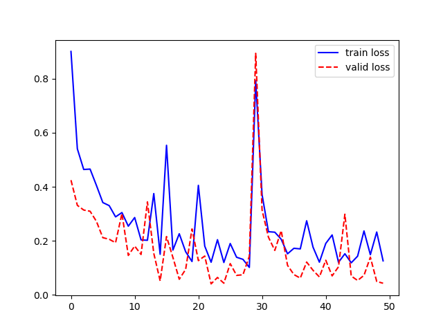
7. 모델 학습

history = model.fit(
    x=x_train,
    y=y_train,
    batch_size=1,
    epochs=50,
    validation_split=0.2,
    verbose=0
)
plt.plot(history.history['loss'], 'b-', label='train loss')
plt.plot(history.history['val_loss'], 'r--', label='valid loss')
plt.legend()
plt.show()

---

8. 모델 검증

loss, acc = model.evaluate(
    x=x_test,
    y=y_test,
    batch_size=1,
    verbose=0
)
print('loss : ', loss)
print('acc : ', acc)
# loss :  0.05600221827626228
# acc :  0.9777777791023254

---

9. 모델 예측값, 실제값 비교

y_pred = model.predict(x_test)
y_pred = np.where(y_pred > 0.5, 1, 0)
print('예측값 : ', y_pred[:4])
print('실제값 : ', y_test[:4])
# 예측값 :  [[0 0 1]
#  [1 0 0]
#  [1 0 0]
#  [0 0 1]]
# 실제값 :  [[0. 0. 1.]
#  [1. 0. 0.]
#  [1. 0. 0.]
#  [0. 0. 1.]]

---

10. 분류모델 성능 평가 - 정확도

acc = accuracy_score(y_test, y_pred)
print('정확도 : ', acc)
# 정확도 :  0.9777777777777777

---

11. 분류모델 종합 성능 평가 - 정확도, 재현도, 정밀도

report = classification_report(y_test, y_pred)
print(report)
#               precision    recall  f1-score   support
#
#            0       1.00      1.00      1.00        15
#            1       1.00      0.93      0.97        15
#            2       0.94      1.00      0.97        15
#
#    micro avg       0.98      0.98      0.98        45
#    macro avg       0.98      0.98      0.98        45
# weighted avg       0.98      0.98      0.98        45
#  samples avg       0.98      0.98      0.98        45

---

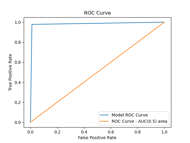
12. ROC 곡선 그리기

FPR, TPR, _ = roc_curve(y_test.flatten(), y_pred.flatten())
auc_value = auc(FPR, TPR)
plt.plot(FPR, TPR, label='Model ROC Curve')
plt.plot([0, 1], [0, 1], label='ROC Curve - AUC(0.5) area')
plt.legend()
plt.title('ROC Curve')
plt.xlabel('False Positive Rate')
plt.ylabel('True Positive Rate')
plt.show()

---

13. AUC 면적값 추출

print('AUC 값 : ', auc_value)
# AUC 값 :  0.9666666666666668