📊 TensorBoard

📌 TensorBoard란?

• 정의
  - 딥러닝 모델 알고리즘 시각화
  - 복잡한 모델의 학습 도중 발생하는 논리적 오류 등을 개선하기 위한 도구

📌 TensorBoard 생성 실습

• 1. 라이브러리 Import

import pandas as pd
import numpy as np
import matplotlib.pyplot as plt
import seaborn as sns
import tensorflow as tf

# StandardScaler(표준화) : 이상치가 있으면 불균형
# MinMaxScaler(정규화) : 이상치에 민감
# RobustScaler : 이상치의 영향을 최소화하는 스케일러
from sklearn.preprocessing import MinMaxScaler, minmax_scale, StandardScaler, RobustScaler

# 학습, 테스트 데이터 분리
from sklearn.model_selection import train_test_split

# Functional API 모델
from keras.models import Model

# Functional API 입력층, Dense층
from keras.layers import Input, Dense

# 텐서보드
from keras.callbacks import TensorBoard

# 회귀모델 성능 지표
from sklearn.metrics import r2_score

---

• 2. 데이터 준비

data = pd.read_csv('../testdata/Advertising.csv')
data = data.iloc[:, 1:]
print(data.head(2))
#       tv  radio  newspaper  sales
# 0  230.1   37.8       69.2   22.1
# 1   44.5   39.3       45.1   10.4

---

• 3. 결측치 확인

print(data.info())
# RangeIndex: 200 entries, 0 to 199
#  #   Column     Non-Null Count  Dtype  
# ---  ------     --------------  -----  
#  0   tv         200 non-null    float64
#  1   radio      200 non-null    float64
#  2   newspaper  200 non-null    float64
#  3   sales      200 non-null    float64

---

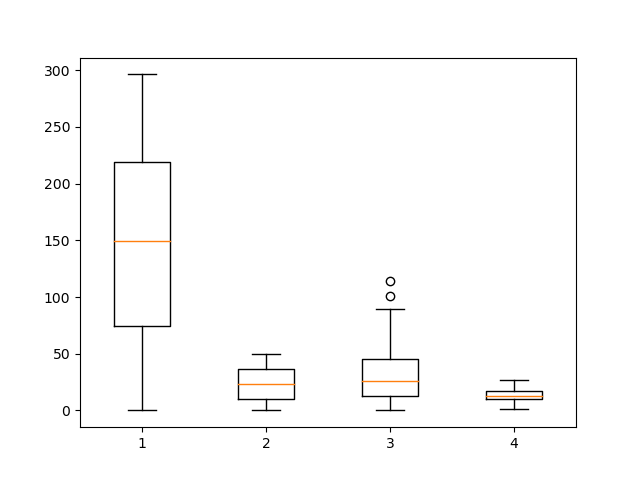
• 4. 이상치 확인

print(data.describe())
#                tv       radio   newspaper       sales
# count  200.000000  200.000000  200.000000  200.000000
# mean   147.042500   23.264000   30.554000   14.022500
# std     85.854236   14.846809   21.778621    5.217457
# min      0.700000    0.000000    0.300000    1.600000
# 25%     74.375000    9.975000   12.750000   10.375000
# 50%    149.750000   22.900000   25.750000   12.900000
# 75%    218.825000   36.525000   45.100000   17.400000
# max    296.400000   49.600000  114.000000   27.000000

plt.boxplot(data)
plt.show()

---

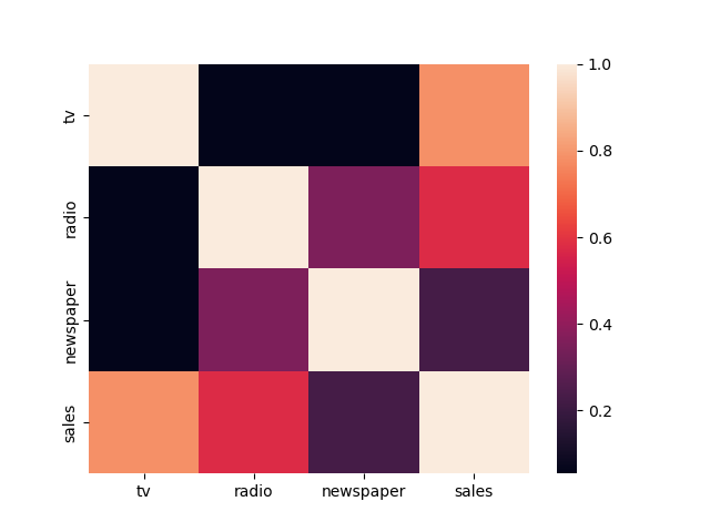
• 5. 상관관계 분석

print(data.corr())
#                  tv     radio  newspaper     sales
# tv         1.000000  0.054809   0.056648  0.782224
# radio      0.054809  1.000000   0.354104  0.576223
# newspaper  0.056648  0.354104   1.000000  0.228299
# sales      0.782224  0.576223   0.228299  1.000000

sns.heatmap(data.corr())
plt.show()

---

• 6. feature, label 분리

feature = data.iloc[:, :-1]
label = data['sales']

---

• 7. feature scaling

# MinMaxScaler
scaler = MinMaxScaler(feature_range=(0, 1))
feature = scaler.fit_transform(feature)
print(feature[:2])
# [[0.77578627 0.76209677 0.60598065]
#  [0.1481231  0.79233871 0.39401935]]

# minmax_scale
# sc_feature = minmax_scale(feature, feature_range=(0, 1), axis=0, copy=True)
# print(sc_feature[:2])
# print(np.array(feature)[:2])
# # [[0.77578627 0.76209677 0.60598065]
# #  [0.1481231  0.79233871 0.39401935]]
# # [[230.1  37.8  69.2]
# #  [ 44.5  39.3  45.1]]

---

• 8. 학습, 테스트 데이터 분리

x_train, x_test, y_train, y_test = train_test_split(feature, label, test_size=0.3, shuffle=True, random_state=123)
print(x_train.shape, x_test.shape, y_train.shape, y_test.shape)
# (140, 3) (60, 3) (140,) (60,)

---

• 9. Functional API 모델 구축

inputs = Input(shape=(3,))
hidden1 = Dense(units=100, activation='relu')(inputs)
hidden2 = Dense(units=50, activation='relu')(hidden1)
outputs = Dense(units=1, activation='linear')(hidden2)

model = Model(inputs, outputs)
print(model.summary())
# Model: "model"
# _________________________________________________________________
#  Layer (type)                Output Shape              Param #   
# =================================================================
#  input_1 (InputLayer)        [(None, 3)]               0         
#
#  dense (Dense)               (None, 100)               400       
#
#  dense_1 (Dense)             (None, 50)                5050      
#
#  dense_2 (Dense)             (None, 1)                 51        
#
# =================================================================
# Total params: 5,501
# Trainable params: 5,501
# Non-trainable params: 0

---

• 10. 모델 학습 최적화 설정

model.compile(optimizer='adam', loss='mse', metrics=['mae'])

---

• 11. 모델 구조 시각화

tf.keras.utils.plot_model(model, 'lin_model.png')

---

• 12. 텐서보드 정의

tb = TensorBoard(
    log_dir='./my',
    histogram_freq=1,
    write_graph=True,
    write_images=False,
    update_freq='epoch',
    profile_batch=2,
    embeddings_freq=1
)

---

• 13. 모델 학습
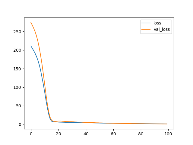
  - validation_split 속성 : 학습 도중 train set에서 validation set을 분리하여 검증을 진행하여 과적합을 예방한다.
  - callbacks 속성 : 콜백함수로 학습 도중 사용하는 하이퍼파라미터이다.

history = model.fit(
    x_train, y_train,
    batch_size=16,
    epochs=100,
    verbose=0,
    validation_split=0.2
)
plt.plot(history.history['loss'], label='loss')
plt.plot(history.history['val_loss'], label='val_loss')
plt.legend()
plt.show()

---

• 14. 텐서보드 실행
  - anaconda prompt 실행
  - 현재 폴더 위치로 이동
  - tnesorboard --logdir my/
  
  

---

• 15. 모델 평가

loss, mae = model.evaluate(x_test, y_test, batch_size=16, verbose=0)
print('loss : ', loss)
print('mae : ', mae)
# loss :  0.6802054643630981
# mae :  0.6597537994384766

---

• 16. 모델 예측값, 실제값 비교

y_pred = model.predict(x_test).flatten()
print('예측값 : ', y_pred[:2])
print('실제값 : ', np.array(y_test)[:2])
# 예측값 :  [11.75939    7.1891627]
# 실제값 :  [11.4  8.8]

---

• 17. 회귀모델 성능 평가 - 설명력

print('설명력 : ', r2_score(y_test, y_pred))
# 설명력 :  0.9823794513514974