
📊 DL 회귀모델 실습
📌 주식 예측 실습
1. 라이브러리 Import
# 기본 라이브러리
import pandas as pd
import numpy as np
import matplotlib.pyplot as plt
import seaborn as sns

# feauture Importance
from sklearn.ensemble import RandomForestRegressor

# 인과관계 분석 라이브러리
from statsmodels.formula.api import ols

# feature scaling
from sklearn.preprocessing import MinMaxScaler

# 학습, 테스트 데이터 분리
from sklearn.model_selection import train_test_split

# 딥러닝 모델
from keras.models import Model
from keras.layers import Input, Dense
from keras.optimizers import Adam

# 회귀모델 성능 지표
from sklearn.metrics import r2_score
2. 데이터 준비
# - 오늘 시가를 이용해 다음날 종가를 예측하는 문제
# - feature는 오늘 데이터
# - label은 내일 데이터
data = pd.read_csv('../testdata/stockdaily.csv')
print(data.head(2))
print(data.shape)
#          Open        High         Low   Volume       Close
# 0  828.659973  833.450012  828.349976  1247700  831.659973
# 1  823.020020  828.070007  821.655029  1597800  828.070007
# (732, 5)

feature = data.iloc[:-1, :-1]
label = data.loc[1:, ['Close']].reset_index(drop=False)
data = pd.concat([feature, label], axis=1)
data.drop(['index'], axis=1, inplace=True)
print(data.head(2))
print(data.shape)
#          Open        High         Low   Volume       Close
# 0  828.659973  833.450012  828.349976  1247700  828.070007
# 1  823.020020  828.070007  821.655029  1597800  824.159973
# (731, 5)
3. feature scaling
col_names = data.columns
feature = data.iloc[:, :-1]
label = data[['Close']]

# feature scaler와 label scaler를 분리
# -> 추후 실제 예측에서 scaling된 예측값을 inverse하기 위해 분리
f_scaler = MinMaxScaler()
l_scaler = MinMaxScaler()
feature = f_scaler.fit_transform(feature)
label = l_scaler.fit_transform(label)
feature = pd.DataFrame(feature)
label = pd.DataFrame(label)
data = pd.concat([feature, label], axis=1)
data.columns = col_names
print(data.head(2))
#        Open      High       Low    Volume     Close
# 0  0.973336  0.975432  1.000000  0.111123  0.977850
# 1  0.956900  0.959881  0.980354  0.142502  0.966455
4. 상관관계 분석
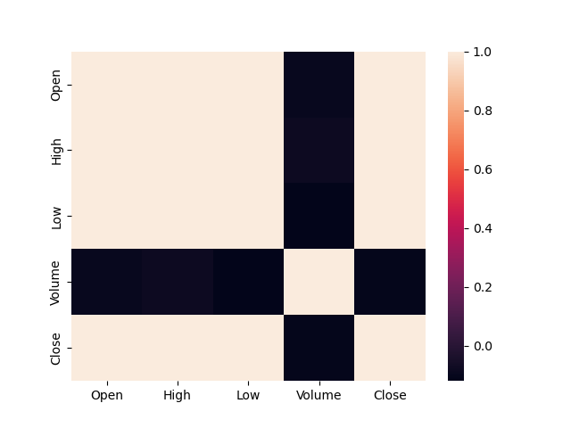
print(data.corr())
#             Open      High       Low    Volume     Close
# Open    1.000000  0.999025  0.998451 -0.094566  0.997916
# High    0.999025  1.000000  0.998335 -0.080936  0.997020
# Low     0.998451  0.998335  1.000000 -0.119666  0.996967
# Volume -0.094566 -0.080936 -0.119666  1.000000 -0.107625
# Close   0.997916  0.997020  0.996967 -0.107625  1.000000

sns.heatmap(data.corr())
plt.show()
# -> Volume과 음의 방향으로 매우 낮은 상관관계를 갖는다.
# -> 추후 feature choose에 있어 참고 자료로 사용 가능
5. feature Importance 확인
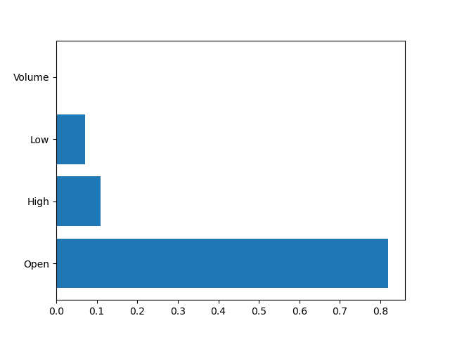
feature = data.iloc[:, :-1]
label = data['Close']
rf = RandomForestRegressor(n_estimators=2000, random_state=1)
rf.fit(feature, label)
plt.barh(y=feature.columns, width=rf.feature_importances_)
plt.show()
# -> Volume 칼럼의 특성 중요도가 매우 낮다.
# -> 추후 feature choose에 있어 참고 자료로 사용 가능
6. 필요 칼럼 추출
data.drop(['Volume'], axis=1, inplace=True)
print(data.head(2))
7. ols 모델을 통해 인과관계 분석
lr = ols(formula='Close ~ Open + High + Low', data=data).fit()
print(lr.summary())
#                             OLS Regression Results
# ==============================================================================
# Dep. Variable:                  Close   R-squared:                       0.996
# Model:                            OLS   Adj. R-squared:                  0.996
# Method:                 Least Squares   F-statistic:                 5.967e+04
# Date:                Thu, 01 Dec 2022   Prob (F-statistic):               0.00
# Time:                        10:38:39   Log-Likelihood:                 1870.8
# No. Observations:                 731   AIC:                            -3734.
# Df Residuals:                     727   BIC:                            -3715.
# Df Model:                           3
# Covariance Type:            nonrobust
# ==============================================================================
#                  coef    std err          t      P>|t|      [0.025      0.975]
# ------------------------------------------------------------------------------
# Intercept      0.0048      0.001      3.559      0.000       0.002       0.007
# Open           0.8423      0.059     14.256      0.000       0.726       0.958
# High          -0.0519      0.057     -0.907      0.364      -0.164       0.060
# Low            0.2062      0.045      4.580      0.000       0.118       0.295
# ==============================================================================
# Omnibus:                      618.301   Durbin-Watson:                   1.972
# Prob(Omnibus):                  0.000   Jarque-Bera (JB):            56123.884
# Skew:                          -3.210   Prob(JB):                         0.00
# Kurtosis:                      45.443   Cond. No.                         143.
# ==============================================================================

# [ ols 모델 summary 결과 분석 ]
# p-value = 0.00 < 0.05(유의수준)
# -> 유의확률이 유의수준 안에 속하므로 모델의 유의성 성립
# feature p-value 중에서 High의 p-value = 0.364 > 0.05(유의수준)
# -> High feature의 유의확률이 유의수준 밖에 존재하므로 해당 feature는 유의한 label을 추출할 수 없다고 판단
# -> High feature의 인과관계가 성립하지 않음
# -> 추후 High feature 선택에 참고 자료로 사용
8. 학습, 테스트 데이터 분리
feature = data.iloc[:, :-1]
label = data['Close']

# 시계열 데이터이므로 shuffle은 False로 지정
x_train, x_test, y_train, y_test = train_test_split(feature, label, test_size=0.3, shuffle=False, random_state=1)
print(x_train.shape, x_test.shape, y_train.shape, y_test.shape)
# (511, 3) (220, 3) (511,) (220,)
9. 딥러닝 모델 구축
inputs = Input(shape=(3,))
hidden1 = Dense(units=300, activation='relu')(inputs)
hidden2 = Dense(units=250, activation='relu')(hidden1)
hidden3 = Dense(units=200, activation='relu')(hidden2)
hidden4 = Dense(units=100, activation='relu')(hidden3)
outputs = Dense(units=1, activation='linear')(hidden4)

model = Model(inputs, outputs)
print(model.summary())
# Model: "model"
# _________________________________________________________________
#  Layer (type)                Output Shape              Param #
# =================================================================
#  input_1 (InputLayer)        [(None, 3)]               0
#
#  dense (Dense)               (None, 300)               1200
#
#  dense_1 (Dense)             (None, 250)               75250
#
#  dense_2 (Dense)             (None, 200)               50200
#
#  dense_3 (Dense)             (None, 100)               20100
#
#  dense_4 (Dense)             (None, 1)                 101
#
# =================================================================
# Total params: 146,851
# Trainable params: 146,851
# Non-trainable params: 0
10. 모델 학습 최적화 설정
model.compile(optimizer=Adam(learning_rate=0.001), loss='mse', metrics=['mae'])
11. 모델 학습 및 학습, 검증 loss 변동률 시각화
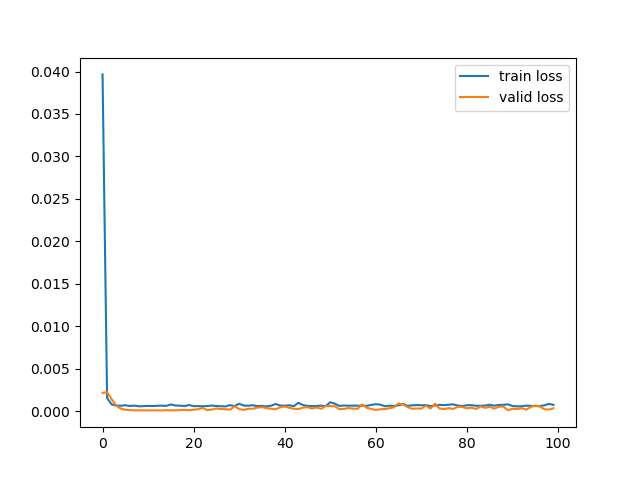
history = model.fit(
    x_train, y_train,
    batch_size=16,
    epochs=100,
    validation_split=0.2,
    verbose=0
)
plt.plot(history.history['loss'], label='train loss')
plt.plot(history.history['val_loss'], label='valid loss')
plt.legend()
plt.show()
12. 모델 검증
loss, mae = model.evaluate(
    x_test, y_test,
    batch_size=16,
    verbose=0
)
print('loss : ', loss)
print('mae : ', mae)
# loss :  0.00033164239721372724
# mae :  0.01409887708723545
13. 모델 예측값, 실제값 비교
y_pred = model.predict(x_test).flatten()
print('예측값 : ', y_pred[:4])
print('실제값 : ', np.array(y_test)[:4])
# 예측값 :  [0.09666555 0.08973867 0.09365381 0.07898248]
# 실제값 :  [0.10282233 0.11206117 0.10209368 0.0880459 ]
14. 회귀모델 성능 지표 - 설명력
print('설명력 : ', r2_score(y_test, y_pred))
# 설명력 :  0.9427100703204642
📊 DL 스킵연결층
📌 DL 스킵연결층이란?
- 정의
- 입력층이나 2단계 이전에 수행한 출력값과 최근 출력값을 Concatenate하는 Layer
- 특징
- 학습 과정으로 인한 수정 데이터는 원본 데이터의 특징을 잃어버릴 수 있다.
- 이를 해결하기 위해 초기 데이터와 최근 출력값을 합쳐 학습 과정 중 데이터의 특징을 유지할 수 있도록 도와준다.
📌 DL 스킵연결층 실습
1. 라이브러리 Import
# 기본 라이브러리
import pandas as pd
import numpy as np
import matplotlib.pyplot as plt
import seaborn as sns

# 데이터세트
from sklearn.datasets import fetch_california_housing

# feature scaling
from sklearn.preprocessing import MinMaxScaler, StandardScaler

# 학습, 테스트 데이터 분리
from sklearn.model_selection import train_test_split

# 딥러닝 모델
from keras.models import Sequential, Model
from keras.layers import Input, Dense, Concatenate
from keras.optimizers import SGD, RMSprop, Adam
from sklearn.semi_supervised.tests.test_self_training import y_train_missing_labels

# 회귀모델 성능 지표
from sklearn.metrics import r2_score
2. 데이터 준비
housing = fetch_california_housing()
feature = pd.DataFrame(housing.data, columns=housing.feature_names)
label = pd.DataFrame(housing.target, columns=housing.target_names)
data = pd.concat([feature, label], axis=1)
print(data.head(2))
#    MedInc  HouseAge  AveRooms  ...  Latitude  Longitude  MedHouseVal
# 0  8.3252      41.0  6.984127  ...     37.88    -122.23        4.526
# 1  8.3014      21.0  6.238137  ...     37.86    -122.22        3.585
3. feature scaling
feature = data.iloc[:, :-1]
label = data[['MedHouseVal']]

f_scaler = MinMaxScaler()
feature = f_scaler.fit_transform(feature)
4. 학습, 테스트 데이터 분리
x_train, x_test, y_train, y_test = train_test_split(feature, label, test_size=0.3, shuffle=True, random_state=1)
print(x_train.shape, x_test.shape, y_train.shape, y_test.shape)
# (14448, 8) (6192, 8) (14448, 1) (6192, 1)
5. 학습, 검증 데이터 분리
x_train, x_valid, y_train, y_valid = train_test_split(x_train, y_train, test_size=0.25, shuffle=True, random_state=1)
print(x_train.shape, x_valid.shape, y_train.shape, y_valid.shape)
# (10836, 8) (3612, 8) (10836, 1) (3612, 1)
6. 딥러닝 모델 구축 - Functional API
input_a = Input(shape=(5,), name='first_input_layer')
input_b = Input(shape=(6,), name='second_input_layer')

net1 = Dense(units=30, activation='relu')(input_b)
net2 = Dense(units=25, activation='relu')(net1)

# 스킵 연결 - 마지막 은닉층 출력과 입력층을 연결함으로써 초기 데이터의 특성을 유지할 수 있음
concat1 = Concatenate()([input_a, net2])

net3 = Dense(units=10, activation='relu')(concat1)
net4 = Dense(units=5, activation='relu')(net3)

# 스킵 연결 - 마지막 은닉층 출력과 입력층을 연결함으로써 초기 데이터의 특성을 유지할 수 있음
concat2 = Concatenate()([concat1, net4])

outputs = Dense(units=1, activation='linear')(concat2)

model = Model(inputs=[input_a, input_b], outputs=outputs)
7. 모델 학습 최적화 방법 설정
model.compile(optimizer=Adam(learning_rate=0.001), loss='mse', metrics=['mae'])
8. 학습, 검증, 테스트 데이터 feature 분리 및 모델 학습
x_train_a, x_train_b = x_train[:, :5], x_train[:, 2:]
x_valid_a, x_valid_b = x_valid[:, :5], x_valid[:, 2:]
x_test_a, x_test_b = x_test[:, :5], x_test[:, 2:]

history = model.fit(
    x=(x_train_a, x_train_b),
    y=y_train,
    batch_size=128,
    epochs=100,
    validation_data=([x_valid_a, x_valid_b], y_valid),
    verbose=0
)
plt.plot(history.history['loss'], label='train loss')
plt.plot(history.history['val_loss'], label='valid loss')
plt.legend()
plt.show()
9. 모델 검증
loss, mae = model.evaluate(
    x=(x_test_a, x_test_b),
    y=y_test,
    batch_size=128,
    verbose=0
)
print('loss : ', loss)
print('mae : ', mae)
# loss :  0.3262670040130615
# mae :  0.3956793248653412
10. 모델 예측값, 실제값 비교
y_pred = model.predict(x=(x_test_a, x_test_b)).flatten()
print('예측값 : ', y_pred[:4])
print('실제값 : ', np.array(y_test).flatten()[:4])
# 예측값 :  [3.5304067 0.6521266 2.7070088 1.6039628]
# 실제값 :  [3.55  0.707 2.294 1.125]
11. 회귀모델 성능 지표 - 설명력
print('설명력 : ', r2_score(y_test, y_pred))
# 설명력 :  0.7351514472888567

데이터 사이언티스트를 목표로 하는 개발자