Linear regression 2 _ abalone

🛻 abalone 데이터에 대해 다음과 같은 것들을 수행한다

• sex가 M인 샘플에 대해, Length와 Height의 회귀선을 긋고, sse값 구하기
• 각각의 sex (M, F) 에 대해, Whole weight 대비, Shucked weight, Vicera weight, Shell weight 의 각 % 구성비 구하기

import numpy as np
import pandas as pd
import matplotlib.pyplot as plt

⌨️ 데이터 준비

url = 'https://archive.ics.uci.edu/ml/machine-learning-databases/abalone/abalone.data'
np_data = pd.read_csv(url,header=None).to_numpy()
print(np_data[:5,],np_data.shape)

# result
# [['M' 0.455 0.365 0.095 0.514 0.2245 0.101 0.15 15]
   ['M' 0.35 0.265 0.09 0.2255 0.0995 0.0485 0.07 7]
   ['F' 0.53 0.42 0.135 0.677 0.2565 0.1415 0.21 9]
   ['M' 0.44 0.365 0.125 0.516 0.2155 0.114 0.155 10]
   ['I' 0.33 0.255 0.08 0.205 0.0895 0.0395 0.055 7]] (4177, 9)

.
.

⌨️ sex가 M인 샘플에 대해, Length와 Height의 회귀선을 긋고, sse값 구하기

• sex가 M인 sample 추출 -> sub_data

filter = np_data[:,0] =='M'

sub_data = np_data[filter]
sub_data[:5]

# result 
# array([['M', 0.455, 0.365, 0.095, 0.514, 0.2245, 0.101, 0.15, 15],
         ['M', 0.35, 0.265, 0.09, 0.2255, 0.0995, 0.0485, 0.07, 7],
         ['M', 0.44, 0.365, 0.125, 0.516, 0.2155, 0.114, 0.155, 10],
         ['M', 0.475, 0.37, 0.125, 0.5095, 0.2165, 0.1125, 0.165, 9],
         ['M', 0.43, 0.35, 0.11, 0.406, 0.1675, 0.081, 0.135, 10]],
      dtype=object)

• Length 와 Height에 대한 회귀선 구하기
  » np.polyfit / np.poly1d 사용

x = sub_data[:,1].astype(np.float64)  # Length
y = sub_data[:,3].astype(np.float64)  # Height

fit_line = np.polyfit(x,y,1)
print(fit_line)

# result
# [ 0.28217804 -0.00703124]

f = np.poly1d(fit_line)
print(f)    # result : 0.2822 x - 0.007031

• 시각화

_, axe = plt.subplots()
axe.scatter(x, y)
axe.plot(x, fit_line[0]*x + fit_line[1], color = "r")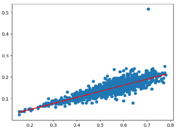

.
.

⌨️ 각각의 sex (M, F) 에 대해, Whole weight 대비 Shucked weight, Vicera weight, Shell weight 의 각 % 구성비 구하기

• sex = M

# sub_data[:,4]  : Whole weight
# sub_data[:,5]  : Shucked weight
# sub_data[:,6]  : Vicera weight
# sub_data[:,7]  : Shell weight

feature_name = ['Shucked','Viscera','Shell']

for i in range(5,8) :
    t = sub_data[:,i] / sub_data[:,4] *100
    print(feature_name[i-5], np.mean(t))
    
    
# result
# Shucked 43.06877369031254
  Viscera 21.85076925029915
  Shell 29.14605543601223

• sex = F

filter = np_data[:, 0] == "F"
sub_data1 = np_data[filter]
sub_data1[:5]

# result
# array([['F', 0.53, 0.42, 0.135, 0.677, 0.2565, 0.1415, 0.21, 9],
         ['F', 0.53, 0.415, 0.15, 0.7775, 0.237, 0.1415, 0.33, 20],
         ['F', 0.545, 0.425, 0.125, 0.768, 0.294, 0.1495, 0.26, 16],
         ['F', 0.55, 0.44, 0.15, 0.8945, 0.3145, 0.151, 0.32, 19],
         ['F', 0.525, 0.38, 0.14, 0.6065, 0.194, 0.1475, 0.21, 14]],
      dtype=object)

feature_name = ['Shucked','Viscera','Shell']

for i in range(5,8) :
    t = sub_data1[:,i] / sub_data1[:,4] *100
    print(feature_name[i-5], np.mean(t))
    
# result 
# Shucked 42.32978625715371
  Viscera 22.136504174282255
  Shell 29.247267809564086