Linear regression 1 _ Iris

🛻 iris 데이터의 회귀선 추정 & matplotlib를 이용한 시각화

import numpy as np
import pandas as pd
import matplotlib.pyplot as plt

⌨️ 데이터 준비

url = 'https://archive.ics.uci.edu/ml/machine-learning-databases/iris/iris.data'
np_data = pd.read_csv(url,header=None).to_numpy()
print(np_data[:5],np_data.shape)

# [[5.1 3.5 1.4 0.2 'Iris-setosa']
#  [4.9 3.0 1.4 0.2 'Iris-setosa']
#  [4.7 3.2 1.3 0.2 'Iris-setosa']
#  [4.6 3.1 1.5 0.2 'Iris-setosa']
#  [5.0 3.6 1.4 0.2 'Iris-setosa']] (150, 5)

iris 데이터는 Setosa, Versicolour, Virginica 총 3개의 calss 에 대한 데이터가 각각 50개씩 있으며, 4개의 attribute가 있는 데이터이다.
.
.

⌨️ Setosa의 sepal length와 sepal width 사이의 회귀선 추정

먼저, 해당 데이터를 sub_data로 들고온다.

sub_data = np_data[:50, [0,1]]

• scatter plot

x = sub_data[:, 0]   #sepal length
y = sub_data[:, 1]   #sepal width

_, axe = plt.subplots()
axe.scatter(x, y)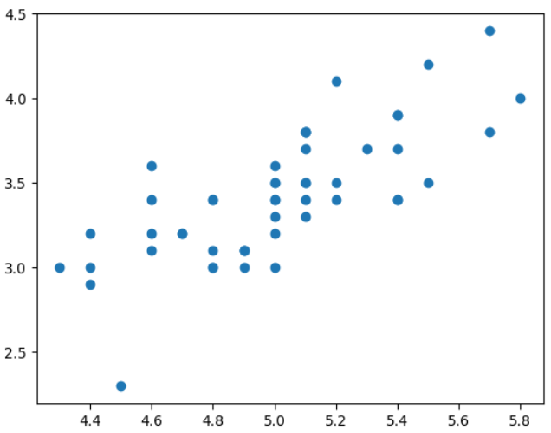

• regression line

‖ np.ployfit
: np.polyfit (독립변수열, 종속변수열, 1)

fit_line = np.polyfit(x, y,1)
print(fit_line)

# result
# [ 0.80723367 -0.62301173]  <- [기울기, y절편]
# y = 0.80723367x - 0.62301173

_, axe = plt.subplots()
axe.scatter(x,y)
axe.plot(x, fit_line[0]*x+fit_line[1], color ="y")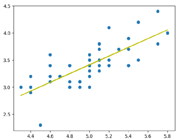

‖ np.poly1d
앞에서 구한 polyfit의 결과값의 객체 fit_line 을 입력해서 함수 f 로 만든다.

f = np.poly1d(fit_line)
print(f)

# result
# 0.8072 x - 0.623

print(f(1))    # result : 0.18422193751847993