
abalone data
import numpy as np
import pandas as pd
import matplotlib.pyplot as plt
from scipy import stats
import statsmodels.api as sm
url = 'https://archive.ics.uci.edu/ml/machine-learning-databases/abalone/abalone.data'
pd_data = pd.read_csv(url, header=None)
#print(pd_data.head())
np_data = pd_data.to_numpy()
.
.
🛻Length : 독립변수 / Diameter : 종속변수
⌨️ plot, regression line
» indep_var (독립변수, x) : Length
» dep_var (종속변수, y) : Diameter
x = np_data[:, 1].astype(np.float64)  # Length
y = np_data[:, 2].astype(np.float64)  # Diameter

fit_line = np.polyfit(x,y,1)  # regresstion line 추정
f = np.poly1d(fit_line)   #
print(f)

# result
# 0.8155 x - 0.01941
_, axe = plt.subplots()
axe.scatter(x,y)
axe.plot(x, fit_line[0]*x + fit_line[1],color="y")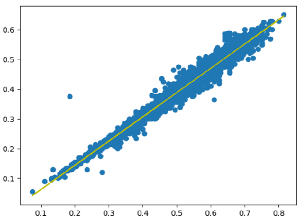
⌨️ statsmodels
- OLS : Ordinary Least Square 함수
x = sm.add_constant(x)   # constant를 계산할 공간을 하나 줘야함.
print(x)

# result
# [[1.    0.455]
   [1.    0.35 ]
   [1.    0.53 ]
   ...
   [1.    0.6  ]
   [1.    0.625]
   [1.    0.71 ]]
reg_model = sm.OLS(y,x)
reg_result = reg_model.fit()
reg_result.summary()
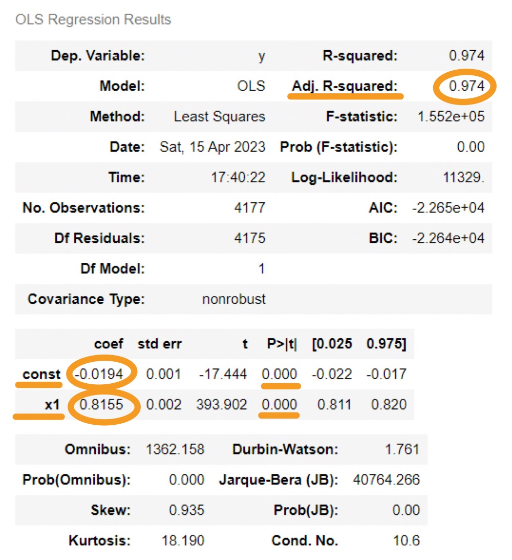
reg_result.params

# result
# array([-0.01941371,  0.81546069]) : [y절편, x계수]

reg_result.rsquared
# result : 0.9737971035056835
.
.
🛻 Length, Diameter, Height : 독립변수 / Rings (나이) : 종속변수
» indep_var (독립변수, x1, x2, x3) : Length(x1), Diameter(x2), Height(x3)
» dep_var (종속변수, y) : Rings
x = np_data[:,1:4].astype(np.float64) # Length, Diameter, Height
y = np_data[:,-1].astype(np.float64)  # Rings (나이)

x = sm.add_constant(x)
reg_result = sm.OLS(y, x).fit()
reg_result.summary()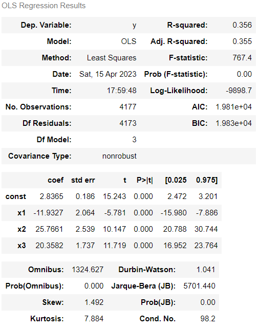
‣ 추정된 회귀식 :
y = 2.8365 - 11.9327×Length +25.7661×Diameter + 20.3582×Height

데이터 분석 / 데이터 사이언티스트 / AI 딥러닝