[Computer Vision] DnCNN
Super Resolution
"Beyond a Gaussian Denoiser: Residual Learning of Deep CNN for Image Denoising"
[Abstract]
DnCNN은 CNN을 이용하여 이미지에서 denoising을 구현한다. 논문에서는 noise의 예시로 Additive White Gaussian Noise(AWGN)을 제거하고자 하였다. 기존의 방식들은 계산 시간이 너무 오래 걸리고, 파라미터 설정에 있어서 복잡한 인간의 개입이 필요한 문제가 있었다. 이 논문에서는 이미지를 직접 denoising하는 것이 아니라 이미지에서 noise를 분리해내는 것에 초점을 맞추었다. 또한 residual learning과 batch normalization을 사용하여 denoising performance를 높였다. 그리고 CNN을 사용하였기 때문에 denoising의 적용에 있어서 유연성을 확보할 수 있었다.
[Key words]
Image Denoising / Convolutional Neural Networks / Residual Learning / Batch Normalization
Residual Learning 장점
- 파라미터를 추가하는 것이 아니므로 계산이 복잡해지지 않음
- 모델이 깊어져도 일반화를 잘 시키며, 정확도를 높임
Batch Normalization 장점
- propagation할 때 parameter의 scale에 영향을 받지 않게 되므로 learning rate을 크게
잡을 수 있어 빠른 학습이 가능함 - 자체적인 regularization 효과가 있어 낮은 민감도를 가짐
The Proposed Denoising CNN Model
일반적으로 specific task를 위해 Deep CNN model을 학습시킬 때 2가지 단계를 가진다.
- 네트워크 구조 디자인
- training data로부터 학습하는 model
저자는 네트워크 구조 디자인을 위해 VGG network를 image denoising에 맞게 변형하였고, sota denoising method에서 사용한 효과적인 patch sizes를 기반으로 network의 depth를 설정하였다. 또한 Model 학습을 위해 Residual learning formulation을 사용했고, 거기에 빠른 학습과 향상된 denoising performance를 위해 Batch normalization을 포함시켰다.
[DnCNN Network Depth]
- Convolution filter size는 3x3이며, pooling layer들은 모두 제거했다. 따라서 depth('d')를 가진 DnCNN의 receptive field는 (2d+1) x (2d+1)이 돼야 한다.
- Denoising neural networks의 receptive field size는 effective patch size와 관련이 있으며, high noise level은 보통 더 많은 context information을 잡아내기 위해 큰 effective patch size를 요구한다. 따라서 저자는 noise level(σ)을 '25'로 고정하고, DnCNN의 depth design을 guide하기 위해 몇몇 leading denoising methods의 effective patch size를 분석했다.
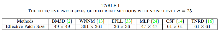
- 위의 표에 있는 Method들은 모두 앞서 설정한 noise level(σ=25)과 다른 effective patch size를 가지고 있었는데 그중 가장 작은 effective patch size를 가진 EPLL(36x36) method를 발견했고, 최종적으로 아래와 같이 설정하여 과연 EPLL과 비슷한 receptive field size를 가진 DnCNN이 leading denoising methds들과 경쟁할 수 있을지 확인하고자 했다.
Image denoising에 맞는 Effective Network Depth 설정
- Convolution filter size : 3x3
- Pooling layer 모두 제거
- DnCNN의 receptive field : (2d + 1) x (2d + 1) *d : depth
- DnCNN의 depth : 17
- DnCNN의 receptive field size : (2x17 + 1) x (2x17 + 1) => 35 x 35
- 다른 일반 image denoising의 depth : 20
[DnCNN Architecture]
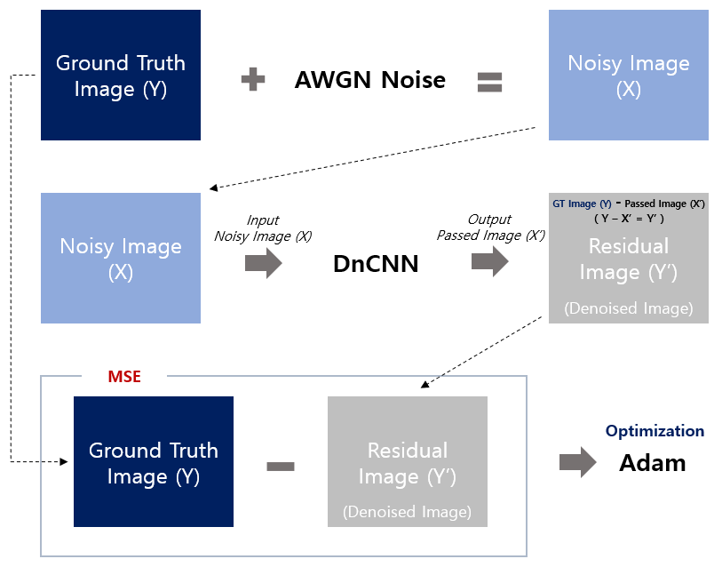
-- DnCNN Architecture Summary --
DnCNN은 기본적으로 CNN을 사용하였다. 우선 Ground truth image(Y)를 구한다. 여기에 AWGN noise를 더하여 Noisy Image X를 만든다. Noisy Image X에 CNN 네트워크를 이용하여 먼저 passed 이미지(X')를 만들고, 원래 이미지(Y)에서 결과 이미지를 감산 연산하여 Residual Image (Y')을 만든다. 최종적으로 Y와 Y'의 MSE를 계산하여 CNN 네트워크의 Optimization에 반영한다.
 또한 Padding에 있어서 단순히 zero padding하는 것으로 기존의 CSF나 TNRD의 가장자리 Artifact문제를 해결하였다.
- DnCNN의 input : Noisy observation (y = x + v)
MLP method나 CSF method와 같은 Discriminative denoising models은 latent clean image를 예측하기 위해 mapping function(F(y) = x)을 학습시키는 것을 목표로 한다. DnCNN은 residual mapping(R(y) ≈ v)을 학습시키기 위해 아래와 같은 Residual learning formulation을 사용하였다.
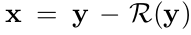
또한 파라미터(Θ)를 학습시키기 위해 loss function으로 일반적인 Mean Squared Error(MSE)를 사용하였다.
R(y)를 학습시키기 위한 Residual learning formulation
- N : noisy-clean training image patch pairs
- R(y) : noisy image을 DnCNN에 넣었을 때 나오는 output, 즉 residual image
- y : noisy image
- x : original clear image
.png)
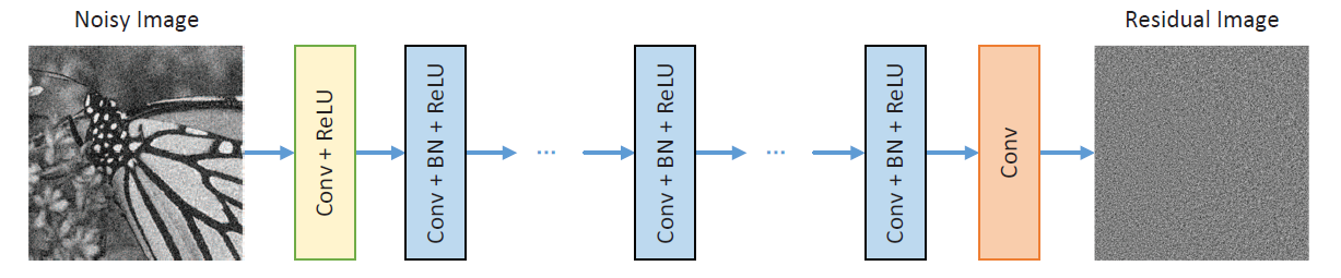
아래 그림은 R(y)를 학습시키기 위해 제안된 DnCNN의 구조이다.
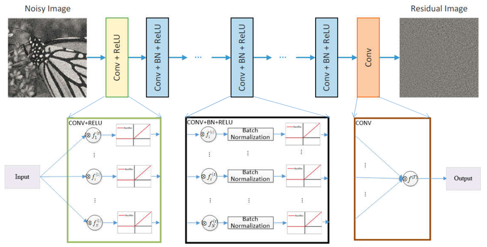
1. Deep Architecture
DnCNN은 세 종류의 layer를 가지고 있다.
1) Conv + ReLU (64 filters of size 3 x 3 x channel)
channel = 3(color image), filter = 64, kernel size = 3- nn.Conv2d(input=3, output=64, kernel_size=3, stride=1, padding=1)
- nn.ReLU()
2) Conv + BN + ReLU (64 filters of size 3 x 3 x 64)
- nn.Conv2d(input=64, output=64, kernel_size=3, padding=1)
- nn.BatchNorm2d(64)
- nn.ReLU()
3) Conv (channel filters of size 3 x 3 x 64)
- nn.Conv2d(input=64, output=3, kernel_size=3, padding=1)
요약하자면, DnCNN 모델은 2개의 주요 특징이 있다.
- R(y)을 학습시키기 위해 Residual learning formulation을 사용한 것.
- 학습 속도와 denoising performance를 향상시키기 위해 Batch normalization을 포함시킨 것.
또한 Convolution에 ReLU를 포함시킴으로써 DnCNN은 hidden layer를 통해 서서히 noisy observation에서 image structure을 분리할 수 있었다.
2. Reducing Boundary Artifacts
많은 low level vision applications은 보통 output image size를 input image size와 같게 유지할 것을 요구하는데, 이로 인해 Boundary artifacts가 생겨날 수 있다.
MLP method에서 noisy input image의 boundary는 preprocessing 단계에서 균형있게 padding을 하는 반면에, CSF method와 TNRD method에서는 모든 단계 전에 padding이 된다.
DnCNN은 이러한 방법들과 다르게 middle layers의 각 feature map들이 계속해서 input image와 같은 사이즈를 가질 수 있도록 convolution 전에 바로 zero padding을 해주었다.
[Integration of Residual Learning and Batch Normalization for Image Denoising]
DnCNN network는 x를 예측하기 위해 original mapping F(y)를 학습시키거나, v를 예측하기 위해 residual mapping R(y)를 학습시키는 데에 사용될 수 있다.
또한 Original mapping이 identity mapping에 더 가까울 때 residual mapping은 더욱 최적화되기 쉽고, Residual learning 관련 논문에 따르면 noisy observation y는 (특히 noise level이 낮을 때) residual image v 보다 latent clean image x에 더 가깝다고 한다.
따라서 R(y)보다 F(y)가 identity mapping에 더 가깝고, residual learning formulation은 image denoising에 더욱 적합하다.
아래의 그래프는 Batch normalization(BN)과 Residual learning(RL)의 사용 유무에 따른 PSNR 평균값을 나타낸 것이다. (Gradient-based optimization 알고리즘으로는 'SGD'와 'Adam'을 사용했다.)
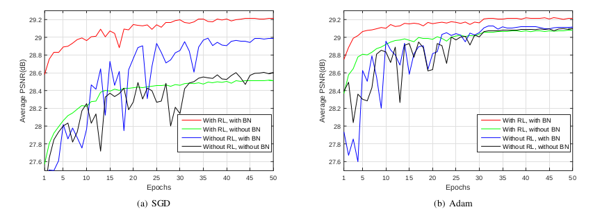
이 그래프를 통해 두 가지 결론을 얻을 수 있다.
- residual learning formulation을 사용할 경우, original mapping learning보다 더 빠르고 안정적으로 수렴된다.
- residual learning formulation과 batch normalizaion을 함께 사용할 경우(Red line), original mapping(Blue line) 보다 빠르게 수렴하고 더 좋은 denoising performance를 나타내는데, 특히 SGD와 Adam optimizaiton algorithms이 이 network가 best 결과를 가질 수 있도록 돕는다.
[Extension to General Image Denoising]
기존의 Gaussian denoising 방법들(MLP, CSF, TNRD)은 fixed noise level을 통해 model을 학습시킨다. 즉, unknown noise에 대해 Gaussian denoising을 할 경우 먼저 noise level을 추정한 후, 이에 해당하는 noise level에 대해 학습된 model을 사용하는 것이 일반적이다.
하지만 이러한 방법들은 accuracy of noise estimation에 영향을 받은 denoising 결과를 나타내게 되며, SISR이나 JPEG deblocking과 같은 non-Gaussian noise distribution에 대해서는 적용될 수 없다.
DnCNN이 unknown noise level에 대해 Gaussian denoising을 가능하게 하도록 wide range of noise levels를 이용해 학습시키고, 학습된 single DnCNN 모델은 test 시 noise level에 대해 estimation 없이 denoise하기 위해 이용될 수 있다.
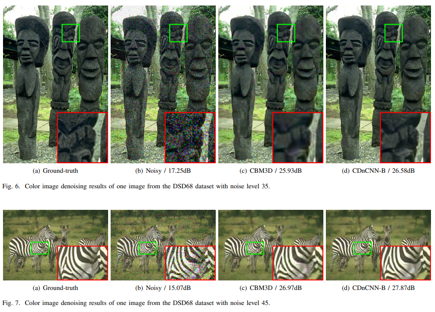
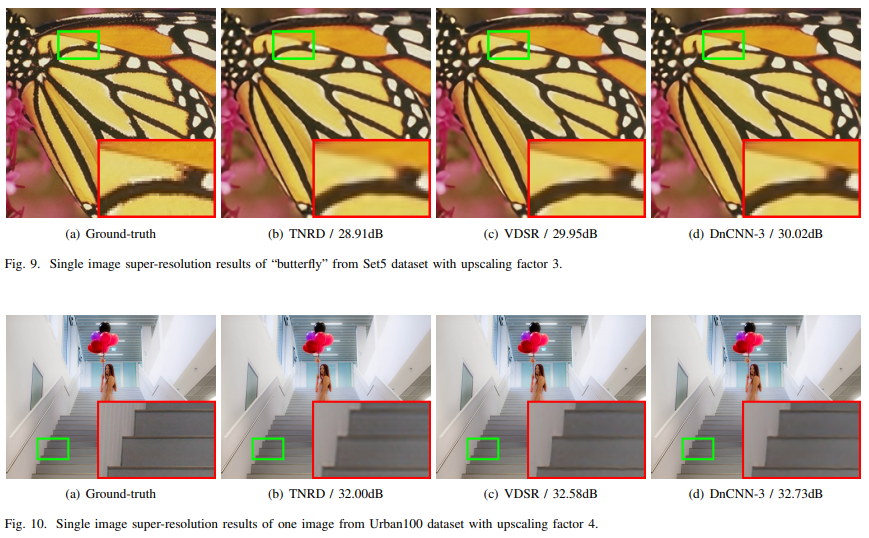
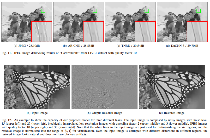
또한, 저자는 몇몇 일반 image denoising tasks에 대해 single DnCNN model을 학습시킴으로써 DnCNN을 더욱 확장시켰는데, blind Gaussian denoing, SISR, JPEG deblocking 이렇게 3가지를 고려하였다.
학습 단계에서 저자는 single DnCNN 모델을 훈련시키기 위해 wide range of noise levels와 multiple upscaling factors가 포함된 down-sampled images, 그리고 다른 quality factors의 JPEG images에게서 받은 AWGN를 포함한 image들을 이용하였고, 실험 결과 several general image denoising tasks(Gaussian denoising, SISR, JPEG deblocking)에서 모두 훌륭한 성능을 보였다.
Result
[Training & Testing data]
-
For Gaussian denoising with either known or unknown noise level
- Train data
: 400 images, size=(180x180) - Training DnCNN-S (known specific noise level)
: noise_levels=(15, 25, 50), patch_size=(40x40), patches=(128x1600) - Training DnCNN-B (blind Gaussian denoising == unknown noise level)
: noise levels=(0~55), patch_size=(50x50), patches=(128x3000) - Test data
: two different test datasets(68 natural iamges from BSD68, 12 images widely used for Gaussian denoising)
- Train data
-
For single model 3 general image denoising tasks
- Train data
: 91 images, 200 images from BSD- Gaussian noise : certain noise of (0~55)
- SISR : bicubic downsampling => bicubic upsampling
- JPEG deblocking : compressing images
- Training DnCNN-3
: patch_size=(50x50), patchs=(128x8000) - Testing : different test set for each task
- Train data
[Parameter Setting]
- Network depth
- DnCNN-S = 17
- DnCNN-B and CnCNN-3 = 20
- Loss function
- Initialize the weights
- SGD with weight decay of 0.0001, momentum of 0.9, mini-batch size of 128
- 50 epochs (learning rate was decayed exponentially from 0.1 to 0.0001 for the 50 epochs)
[Training]
우선 이미지를 준비한다. 본 논문에서는 gray 이미지를 대상으로 함으로 이미지를 우선 gray로 만드는 과정이 필요하다. 그런 다음 Additve White Gaussian Noise를 더하여 noise 이미지를 만든다. 이후 noise가 더해진 이미지에 normalization을 통해서 이미지의 color 값을 0과 1사이로 normalization한다. 학습을 위해서 많은 양의 데이터가 이용될 수 있지만, 논문에 서술되어 있기를 적당한 지점부터는 noise의 MSE가 줄어들지 않음으로, 적당한 데이터의 양이 필요해 보인다.
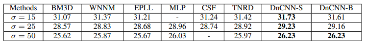
[Quantitative and Qualitative Evaluation]
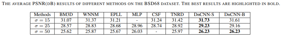
DnCNN-S와 DnCNN-B 모두 다른 competing method들 보다 높은 PSNR 결과를 나타냈는데, 그중 unknown noise level에 대한 모델인 DnCNN-B의 결과가 주목할 만하다.
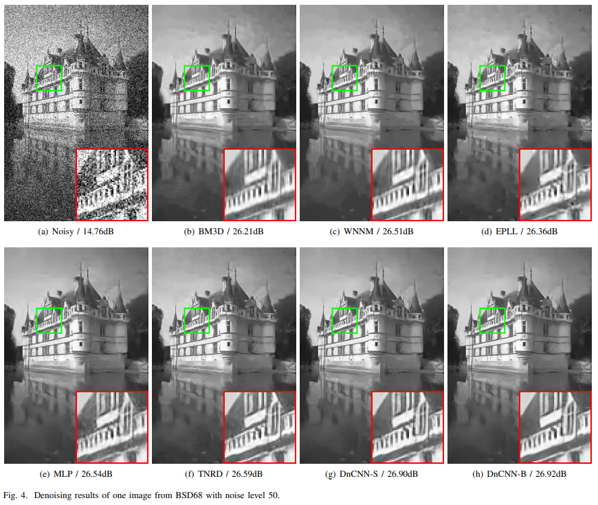

[Conclusion]
결과적으로 노이즈의 크기가 커질수록 DNCNN이 BM3D보다 좋아졌으며, BM3D와는 다르게, DnCNN은 원래의 이미지의 high frequency 부분 (가장자리나 엣지와 같은 특징점)을 보존하려는 경향을 보이고 있었다.
DnCNN을 이용하면, 기존의 방식과는 다르게 다양한 종류의 Noise에 적용할 수 있으며, denoising뿐만 아니라 super resolution같은 분야에도 적용할 수 있어서 유연성면에서 기존의 방식과 차별화를 둘 수 있다. 또한 DnCNN은 BM3D의 blur문제를 많이 감소시켰지만 아직도 Blur문제는 적게나마 남아 있어서 추후 연구에 있어서 이러한 문제를 해결하는 과정이 필요해 보인다. 또한 BM3D와 같이 non local mean과 같은 방식이 사용되지 않았는데, DnCNN에 이러한 방식을 적용한다면 좀더 성능을 높일 수 있어 보였다.

3개의 댓글

Exploring the various types of software development opens up a world of possibilities, from creating immersive video games to developing robust cybersecurity systems. Each type offers unique challenges and opportunities, showcasing the diverse skill sets required in this dynamic field. Whether you're interested in web development, mobile apps, or artificial intelligence, there's a niche for every passion and talent in the software development landscape.https://triberr.com/brian969
Exploring the various types of software development opens up a world of possibilities, from creating immersive video games to developing robust cybersecurity systems. Each type offers unique challenges and opportunities, showcasing the diverse skill sets required in this dynamic field. Whether you're interested in web development, mobile apps, or artificial intelligence, there's a niche for every passion and talent in the software development landscape.https://triberr.com/brian969
Exploring the various types of software development opens up a world of possibilities, from creating immersive video games to developing robust cybersecurity systems. Each type offers unique challenges and opportunities, showcasing the diverse skill sets required in this dynamic field. Whether you're interested in web development, mobile apps, or artificial intelligence, there's a niche for every passion and talent in the software development landscape.