한줄요약

이 논문의 모델인 PANE-GNN은 negative feedback을 constrasitve learning으로 학습한 것을 바탕으로 user가 싫어할만한 items를 추천 목록에서 제외하고, positive feedback을 GNN과 MLP를 통해 학습하여 제외되지 않은 items의 rank를 매기고 추천을 해주는 모델이다.

ABSTRACT

GNN 기반 추천시스템 모델은 negative feedback을 간과하고 positive feedback에만 초점을 맞추고 있다. 이 논문에서는 positive edges와 negative edges를 통합하는 PANE-GNN이라는 모델을 소개한다. user의 preference와 dispreference를 통합하면서 추천 성능을 향상한다. PANE-GNN은 raw rating graph를 positive feedback graph와 negative feedback graph로 분할한다. 그 이후에 positive feedback graph에서는 interest embedding을 얻고, negative feedback graph에서는 disinterest embedding을 얻는다. 효과적인 information propagation을 위해 distinct message-passing mechanisms을 설계하고, contrastive training을 위한 negative graph에서 80%의 edges를 제거한 distortion negative graph를 소개한다. 이 distortion은 negative feedback을 ranking에서 효과적으로 제거하는데 중요한 역할을 수행한다. PANE-GNN은 모든 dataset과 모든 구간에서 SOTA를 기록한다.

1 INTRODUCTION

Observation 1: GNN은 negative feedbackd의 information을 제대로 통합하지 못한다. 이러한 제한은 추천시스템에서 valuable한 user feedback의 활용을 방해한다.

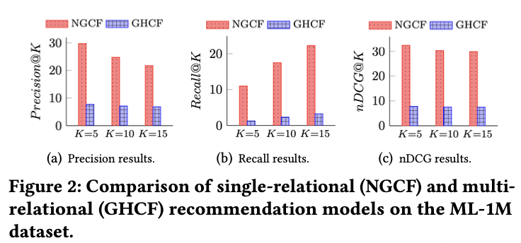
Observation 2: multiple-behavioral graph를 통해 negative feedback을 통합하는 것은 자연스러운 접근으로 보이지만 GHCF로 실험한 결과 negative feedback을 활용하지 않는 NGCF보다 성능이 낮았다 (아래 그림 참고). 이것으로 보았을 때 negative feedback을 직접 통합한다는 것이 항상 이득을 볼 수 있는 것은 아니다.

Challenges: signed bipartite graph에서 high-order structural information을 배우는 것은 network homophily assumption과 balance theory assumption의 한계로 어려움에 직면해있다.

• network homophily assumption은 similar node가 dissimilar node보다 서로 연결될 가능성이 높다고 가정한다. 그러나 homophily는 dissimilar node가 negative edge로 연결된 signed graph에서는 적용되지 않는다.
• balance theory assumption은 "the friend of my friend is my friend", "the enemy of my friend is my enemy", "the enemy of my enemy is my friend"를 가정한다. signed unipartite graph는 이 가정을 활용할 수 있지만, signed partite graph에서는 balance theory assumption가 맞지 않는다. 예를 들어 "내 적의 적은 내 친구이다"라는 가정은 "동일한 user가 싫어하는 두개의 item은 유사하다"로 표현될 수 있는데 이것은 성립할 수 없다. 그래서 real-world의 복잡성을 캡쳐하지 못한다는 것이다.

이러한 제한들은 signed bipartite graph의 독특한 특성과 real-world에서 user의 다양한 interest를 고려하여 추천시스템에서 negative feedback을 효과적으로 활용하기 위한 새로운 접근 방식의 개발을 필요로 한다.

Our idea: 핵심 아이디어는 positive graph와 negative graph의 high-dorder structural information을 모두 활용하는 것이다. negative feedback을 통합하여 추천 성능을 향상 시키기 위해 PANE-GNN이라는 모델을 만들었다. 이 모델은 interest embedding과 disinterest embedding을 만든다. network homophily assumption으로 positive graph에서 interest embedding은 user의 interest를 포착하고, negative graph에서 disinterest embedding은 user의 disinterest를 포착한다. 더 나아가서 graph perturbation에 변하지 않는 robust한 embedding을 만들기 위해서 negative graph와 negative graph의 perturbed version으로 contrastive learning을 한다. 이것은 noise가 있을 때 관련 패턴을 capture하는 모델의 능력을 향상시킨다.

main contributions

• PANE-GNN이라는 새로운 GNN 기반 추천 모델을 제안한다. 이 모델은 positive graph와 negative graph 모두에서 message passing을 수행하여 positive feedback과 negative feedback을 효과적으로 통합한다.
• contrastive learning on the negative graph, new ranking method with a disinterest-score filter, dual feedback-aware Bayesian personalized ranking loss은 모두 positive feedback과 negative feedback 시그널의 통합을 통해 추천 정확도를 향상시킨다.
• PANE-GNN은 모든 dataset, 모든 구간에서 SOTA를 기록한다.

2 RELATED WORK

• Recommender Systems based on GNNs
• Graph Neural Networks on Signed Graphs
  - SiReN

3 METHOD

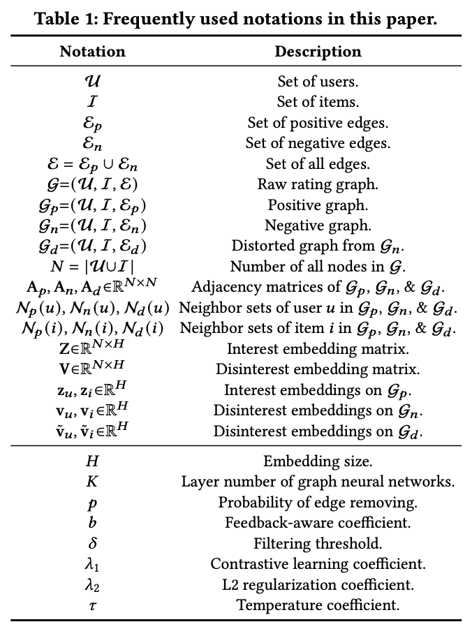
notations는 아래 표와 같다.

three key technical designs
1. message passing on the positive graph G𝑝 and the negative graph G𝑛
2. contrastive learning on the negative graph G𝑛
3. ranking with a disinterest-score filter

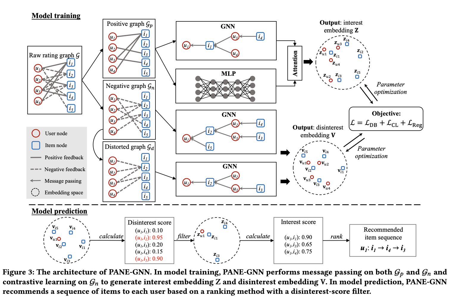
PANE-GNN 모델 architecture는 아래 그림과 같다.

Message passing on G𝑝 and G𝑛
여기서는 interest embeddings과 disinterest embeddings을 얻는다. interest embeddings는 liking and being liked 사이의 관계를 capture하고, disinterest embeddings는 disliking and being disliked 사이의 관계를 capture한다. 그리고 이러한 embedding을 효과적으로 얻기 위해 LightGCN을 이용한다 (LightGCN을 모르면 다음 과정들을 이해하기 힘드니 LightGCN을 필수로 이해하고 와야함. https://arxiv.org/abs/2002.02126). 자세한 수식은 아래와 같다 (모르는 notaion이 있으면 위에 표를 참고하면 된다).
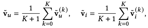
z는 interest embedding이다.

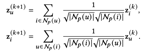
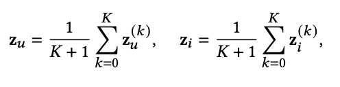
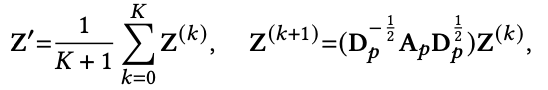
이것을 matrix forms으로 바꾼 것은 아래와 같다.

v는 disinterest embedding이다.

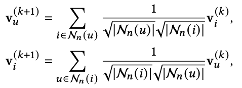
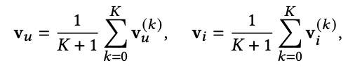
이것을 matrix forms으로 바꾼 것은 아래와 같다. 이렇게 해서 Z'이 나온다.

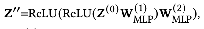
dense한 non-graph information을 모델에 통합하기 위해 이 모델에서는 two-layer MLP를 아래와 같이 사용한다. 이렇게 해서 Z''이 나온다.

이제 Z'과 Z''의 importance를 결정해야한다. 그래서 여기서 attention mechanism을 사용한다. 아래와 같이 𝛼1과 𝛼2를 구하고 이를 활용하여 최종 Z를 얻는다.

Contrastive learning on G𝑛
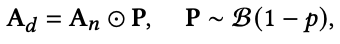
positive feedback은 user의 interest에 대한 신뢰성 있는 지표 역할을 한다. 하지만 negative feedback은 positive feedback에 비해 more susceptible to timeliness하고 contains more noise하다. 이것을 해결하기 위해 여기서는 G𝑛을 distorting한 G𝑑를 만들고, G𝑛과 G𝑑에 contrastive learning을 적용한다. 이 접근 방식은 graph contrastive learning에서 널리 사용되는 data augmentation 전략인 edge 제거를 G𝑛의 adjacency matrix A𝑛에 적용하여 modified adjacency matrix A𝑑를 생성함으로써 수행된다. A𝑑는 아래 식과 같이 만들어진다. 여기서 P는 random masking matrix이다. 이것은 parameter가 p인 Bernoulli 분포를 따른다.

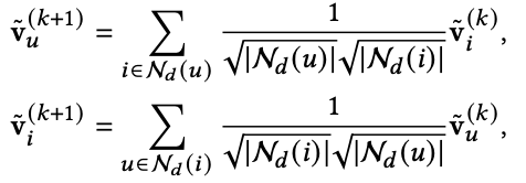
이렇게 만들어진 G𝑑도 G𝑝와 G𝑛처럼 같은 훈련 방식을 아래와 같이 따른다.
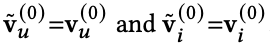
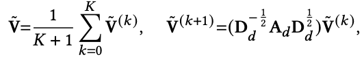여기서 참고적으로 random으로 초기화된 값은 아래와 같다는 것을 알아두자.

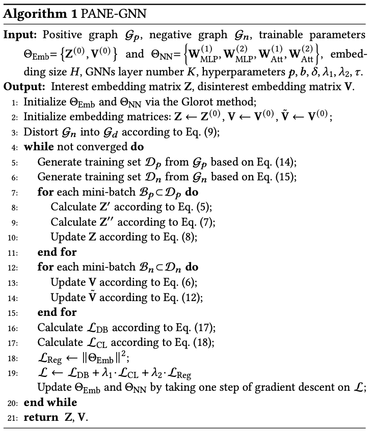
PANE-GNN의 algorithm은 아래와 같다.

Ranking with a disinterest-score filter
interest score 𝑆it와 disinterest score 𝑆dt는 아래와 같이 계산된다.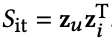 𝑆it (여기서 it는 내 추측에 interest에서 가져온게 아닐까 싶다)는 interest embeddings을 기반으로 user u와 item i 사이의 affinity를 나타낸다.
𝑆dt (여기서 it는 내 추측에 disinterest에서 가져온게 아닐까 싶다)는 disinterest embeddings을 기반으로 user u와 item i 사이의 disinterest or negative affinity를 나타낸다.

user u에 대한 최종 추천 결과는 filtering function Filter(·)와 ranking function Rank(·)로 결정된다.

• filtering function Filter(·): 𝑆dt < threshold 𝛿 의 조건을 만족하는 것만 추천으로 고려되도록 한다. 𝑆dt가 높다는 것은 disinterest가 높다는 것이므로 여기서 설정한 기준보다 높으면 추천 후보군에 올리지 않겠다는 말이다.
• ranking function Rank(·): 위에서 걸러진 것들은 제외하고 나머지들 중에서 (disinterest가 높지 않은 것들 중에서) 𝑆it를 기반으로 rank를 매긴다.

위의 단계들을 결합하여 user u에 대한 최종 추천 결과를 아래와 같이 나타낼 수 있다.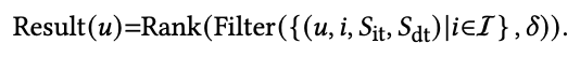

Optimization
G𝑝와 G𝑛의 training set D𝑝와 D𝑛을 아래와 같이 구성한다. notations는 위에 표에 나와있다.

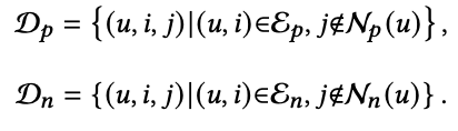
그리고 D𝑝와 D𝑛의 mini-batch B𝑝와 B𝑛을 아래와 같이 둔다.

PANE-GNN의 trainable parameter group은 2개가 있다. 그 2개는 아래와 같다.

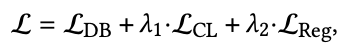
그리고 overall loss function L은 아래와 같다.

L_DB loss
G𝑝와 G𝑛 모두의 information을 통합하기 위해 BPR에서 영감을 받아 만든 dual feedback-aware BPR loss를 활용한다. 식은 아래와 같다.
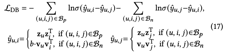여기서 b (b>1, b에 대해서는 section 4에 나옴)는 다음과 같은 priority order를 보장해준다: positive feedback > negative feedback > no feedback.

L_CL loss
InfoNCE loss을 통해 G𝑛에 대한 contrastive objective L_CL을 만든다. 식은 아래와 같다 (InfoNCE loss를 모른다면 관련 내용 찾아봐야 합니다).
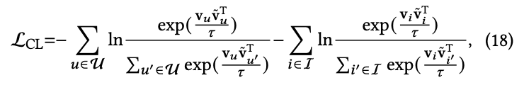여기서 𝜏 (𝜏에 대해서는 section 4에 나옴)는 temperature coefficient이다. 이 loss에서는 contrastive learning framework를 활용하여 disinterest embedding의 robustness와 discriminative power를 향상시킨다.

4 EXPERIMENT

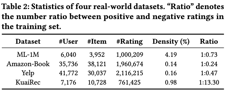
Datasets

• ML-1M
• Amazon-Book
• Yelp
• KuaiRec
  

Baselines

• NGCF
• LR-GCCF
• LightGCN
• SGCN
• SiReN(https://velog.io/@chwchong/SiReN-Sign-Aware-Recommendation-Using-Graph-Neural-Networks)

Metrics

• precision@K
• Recall@K
• nDCG@K

Hyperparameter Setups
hyperparameter를 어떤 값으로 두었는지를 설명하는 subsection이다.
(크게 리뷰할 것은 없어서 hyperparameter들이 어떤 값으로 설정되어서 훈련되는지 자세히 알고 싶다면 논문을 참고하면 좋을 것 같다)

Experimental Results

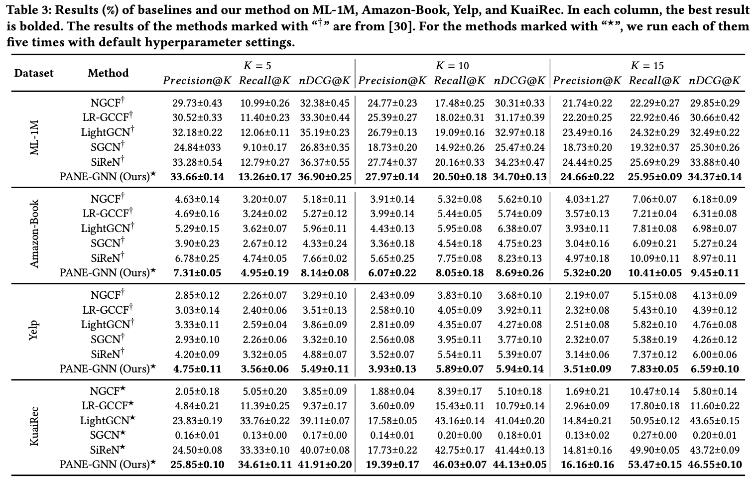
• RQ1: Does PANE-GNN improve overall recommendation performance compared to other GNN-based methods?
  PANE-GNN은 모든 dataset, 모든 구간에서 SOTA를 차지한다. 특히 KuaiRec처럼 positive feedback의 수가 negative feedback의 수보다 작은 dataset을 다룰 때 PANE-GNN의 이점을 강조한다. negative feedback을 활용하는 SiReN과의 비교에서도 확실히 좋은 성능을 보인다. balance theory assumption에 의존하는 SGCN은 다른 방법에 비해 제대로 작동하지 않는다. 이것은 signed unipartite graph를 위해 설계된 balance theory assumption이 user가 일반적으로 다양한 관심사를 가지고 있는 실제 추천 시나리오에 적합하지 않다는 것을 시사한다.
  

• RQ2: How do different components in PANE-GNN affect its performance?
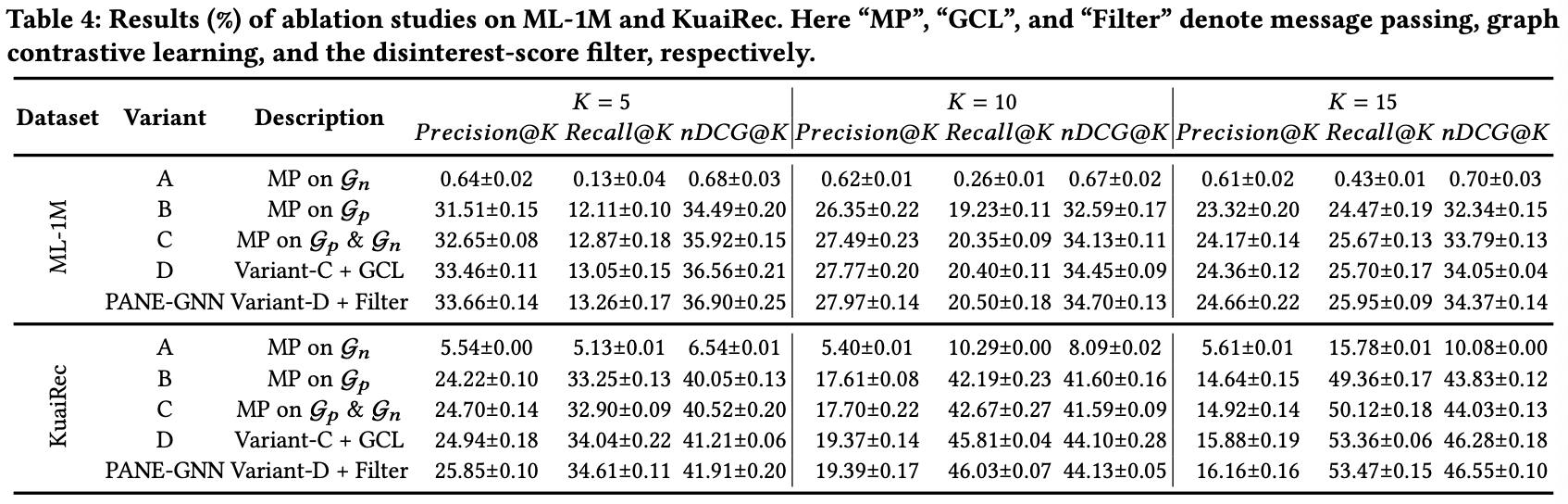
  Ablation studies
  -Variant-A: Using message passing on the negative graph G𝑛.
  -Variant-B: Using message passing on the positive graph G𝑝.
  -Variant-C: Using message passing on both G𝑝 and G𝑛.
  -Variant-D: Introducing graph contrastive learning on Variant-C.
  Variant-A 는 가장 성능이 낮았다. positive feedback이 user의 interest를 인식하는데 중요하다는 것을 의미하고, negative feedback이 이것을 대체할 수는 없다고 한다. 다만 그렇다고해서 negative feedback이 필요없다는 것이 아니라 negative feedback은 user의 disinterest를 인식하는데 도움을 줘야한다.
  Variant-B vs Variant-C 에서는 Variant-C 의 성능이 더 잘나왔다. 이것은 negative graph를 통합하면 성능이 향상된다는 것을 의미한다.
  Variant-C vs Variant-D 에서는 Variant-D 의 성능이 더 높다. 이것은 negative graph에서 disinterest embedding을 배우기 위한 contrastive learning의 효과를 보여준다.
  Variant-D vs PANE-GNN 에서는 PANE-GNN이 더 높게 나온다. 이것은 disinterest score의 정확성과 disintereset-score filter의 효과를 확인시켜준다.
  이 결과는 아래 성능 표에 나와있다.
  

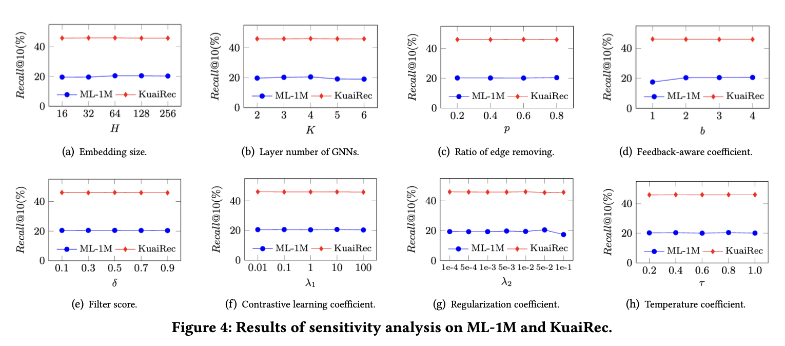
• RQ3: How robust is PANE-GNN in terms of different hyperparameters?
  -GNNs layer number K: 너무 크게 잡으면 over-smoothing 현상이 발생한다.
  -Feedback-aware coefficient b: ML-1M에서 b=1이면 성능이 많이 떨어진다. 이것은 negative feedback과 positive feedback을 구분하는 것이 중요하다는 것을 의미한다. KuaiRec에서는 b=1일 때 성능이 괜찮은데, 이것은 dataset 특성상 negative feedback과 positive feedback을 구분하는 중요성이 감소할 수 있다는 점을 시사한다.
  -Regularization coefficient 𝜆2: 𝜆2=0.1일 때의 성능이 너무 안 좋다. 𝜆2가 너무 크면 underfitting을 초래할 수 있다.
  -Others: 다른 hyperparameters는 값을 바꿔도 큰 변화가 없다. 이것은 PANE-GNN의 robustness를 보여준다.
  실험 결과는 아래와 같다.
  

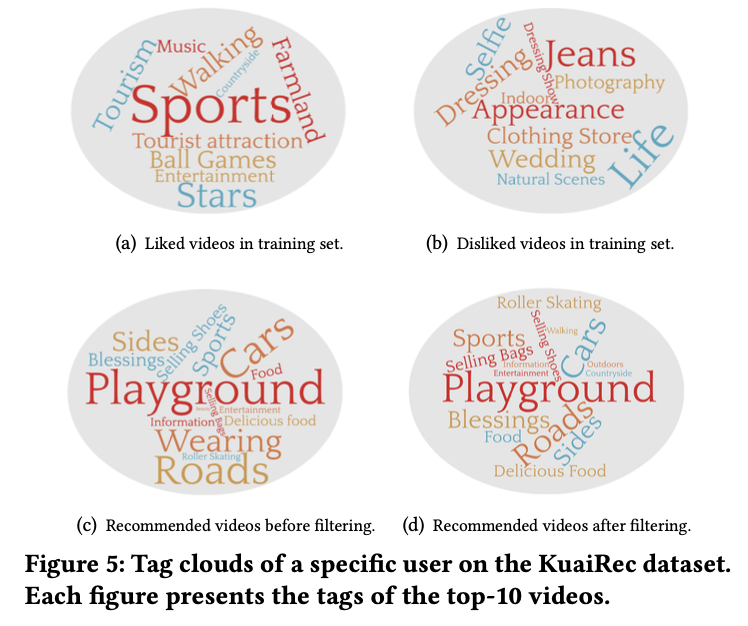
• RQ4: What are the final recommendation results of PANE-GNN from a qualitative perspective?
  아래의 그림은 PANE-GNN의 힘을 하나의 사진으로 보여준다. PANE-GNN은 training data에서 user의 interest과 diinterest을 효과적으로 capture한다 (Figure 5-(a), Figure 5-(b)). 그리고 disinterest-score filter (Figure 5-(c))를 통해 user의 disinterest item을 걸러내고, 최종 추천 (Figure 5-(d))를 한다. 다른 모델과 이 모델의 차별점은 Figure 5-(c)라고 생각한다 (나도 negative feedback 연구하면서 생각했던 이상적인 모델이 PANE-GNN과 유사하다. 특히 user의 disinterest를 걸러내는 filtering 작업이 그렇다).
  

5 CONCLUSION AND FUTURE WORK

이 논문에서 추천시스템을 개선하기 위해 negative feedback을 활용합니다. 그래서 PANE-GNN이라는 모델을 소개하는데, 이 모델은 positive feedback과 negative feeback 모두에서 high-order structural infromation을 capture한다. 그리고 negative graph에 대한 contrastive learning을 사용하여 noise를 줄이고 disinterest score가 높은 items를 필터링하여 추천 결과의 관련성을 보장한다. 이 모델은 모든 dataset과 모든 구간에서 SOTA를 기록한다. 이 논문 저자들은 향후에 GNN 기반 추천 모델에서 노출 편향 문제를 조사할 계획이라고 한다.

code

https://reurl.cc/0ELqO6