Model에 plug in 하여 광범위한 문제에 걸쳐서 잘 동작하도록 하는 best building blocks를 찾을 것이다.
Recurrent model의 문제
🔗 Linear interaction distance
- RNNs는 linear locality를 encode한다.
- 근처에 있는 word들은 서로의 meaning에 영향을 끼친다.
- 하지만 word들이 linearly하게 멀리 떨어져 있어도 여전히 interact하는 경우가 있다.
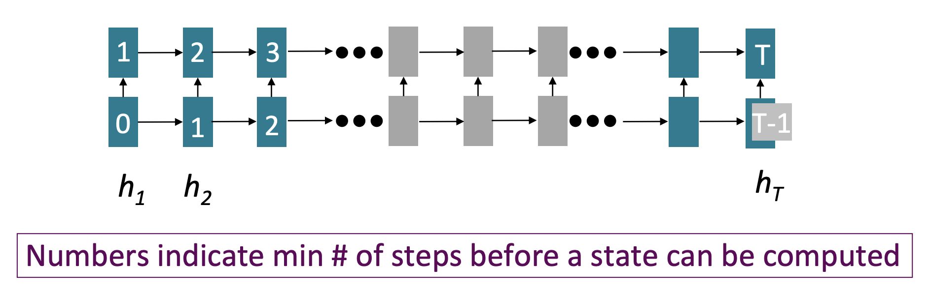
✔️ Problem : RNNs에서는 멀리 떨어져 있는 word쌍이 interact하려면 O(sequence length) steps가 걸린다.
- 따라서 gradient problem때문에, long-distance dependencies를 학습하기 어렵다.
- LSTM이 simple RNN보다 gradient를 잘 propagate하지만, 완벽하진 않다.
- Linear order가 sentence에 대해 생각하는 올바른 방법이 아니라는 것을 알고있다.
🔗 Lack of parallelizability
✔️ Forward와 backward pass가 O(sequence length)의 unparallelizable operations를 가지고 있다.
- GPU는 a bunch of independent computations를 한번에 수행할 수 있다. ➡️ Paralleizability
- 하지만 RNN에서는 한 번에 할 수 없다. Recurrent equations 안에 명시적인 time dependence가 있기 때문이다. 그래서 time dimension에 대해 parallelize할 수 없다.
- 매우 큰 datasets에 대해 training하는 것을 못하게 한다.
모델의 reccurrence와 직접 관련이 있다. 매우 유용하다고 생각했던 것이 지금은 problematic한 원인이 되었다.
➡️ Recurrence를 building block 그 자체로 대체하고 싶다.
그렇다면 word windows는 어떨까?
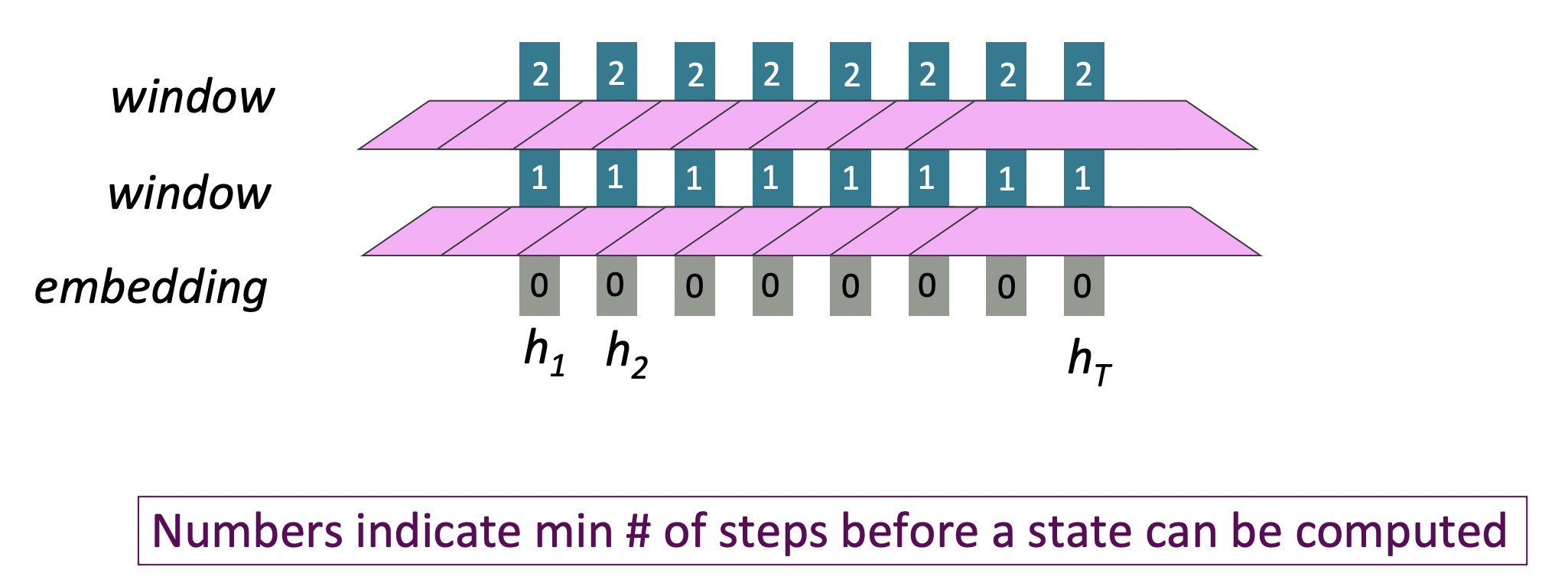
Word models는 local contexts를 모은다. 의 local window는 time과 independent하게 볼 수 있다.
- Parallelizable할 수 없는 operation의 수가 sequence length와 함께 증가하지 않는다. O(1)
- Maximum Interaction distance = sequence length/window size
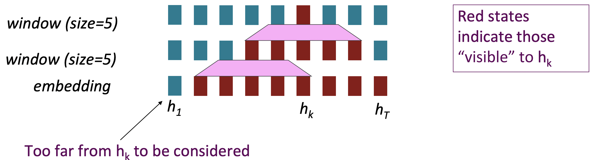
문제는, long-distance dependencies를 학습할 수 있느냐이다. 물론 word window layers를 쌓아서 interaction할 수 있는 거리를 늘릴 수는 있지만, 여전히 항상 finite field이다.
그렇다면 attention은 어떨까?
Attention은 각 word의 representation을 access하기 위한 query로 취급하고, a set of values에서 정보를 통합시킨다. 지금은 single sentence 내에서의 attention에 대해 생각해본다.
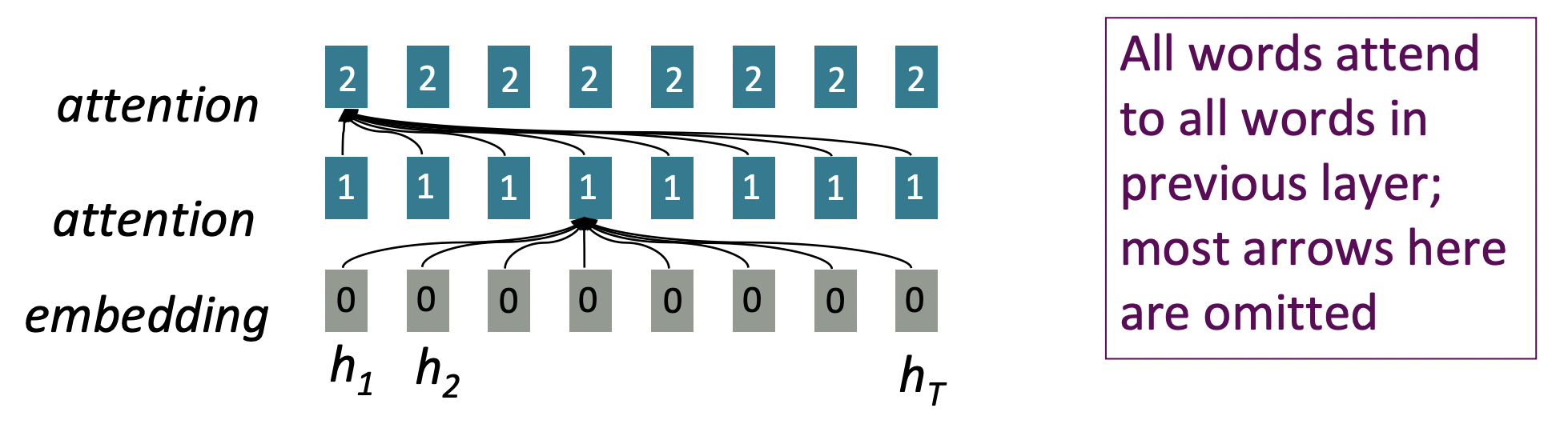
- Parallelizable할 수 없는 operation의 수가 sequence length와 함께 증가하지 않는다. O(1)
- Depth에 관해서는 parallelize할 수 없는데, time에 관해서는 parallelize할 수 있다.
- Maximum interaction distance: O(1), 모든 layer에서 모든 word가 interact한다.
- Recurrent neural network에서는 O(t) operations가 필요했는데, attention으로는 즉시 interact한다.
Self-Attention
-
Attention은 queries, keys, 그리고 values에 대해 동작한다.
-
queries : , , ... , . 각 query 는 R^d vector
-
keys : , , ... , . 각 key 는 R^d vector
-
values : , , ... , . 각 value 는 R^d vector
여기서는 query, key, value의 개수가 같지만, 실제로는 query의 수는 key와 value의 수와 다를 수 있다.
-
-
Self-attention에서는, queries, keys, values가 same source(ex. same sentence)에서 나온다.
- = = =
-
(dot product) Self-attention operation은 다음과 같다:
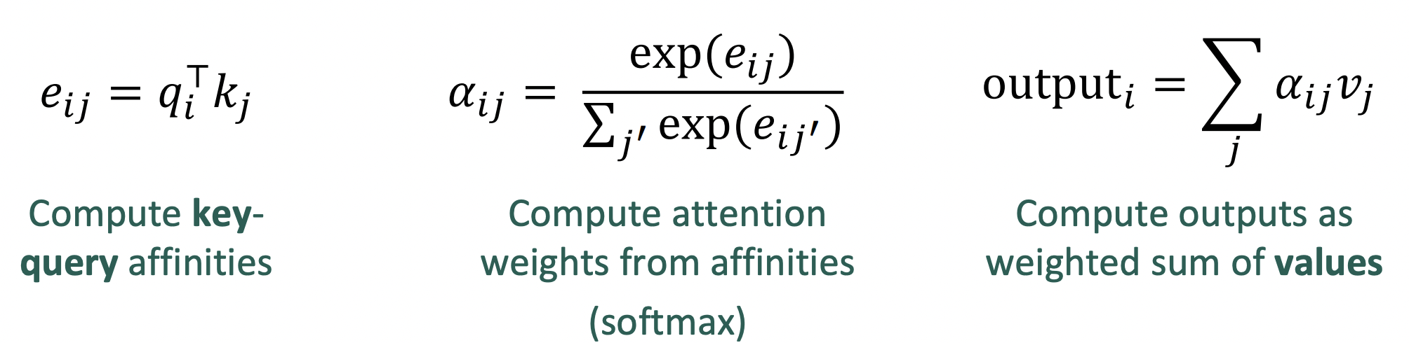
- e_ij : T by T matrix (친화력)
- α_ij : attention weight
- 분모 : summing over all of the keys
- 분자 : where should this query be looking?
- : one output for one query
❓ Fully-connected layer와 다른점
- interaction weights를 학습할 수 있다.
- dynamic connectivity를 가진다.
🔗 Self-attention을 building block으로 보았을 때의 문제
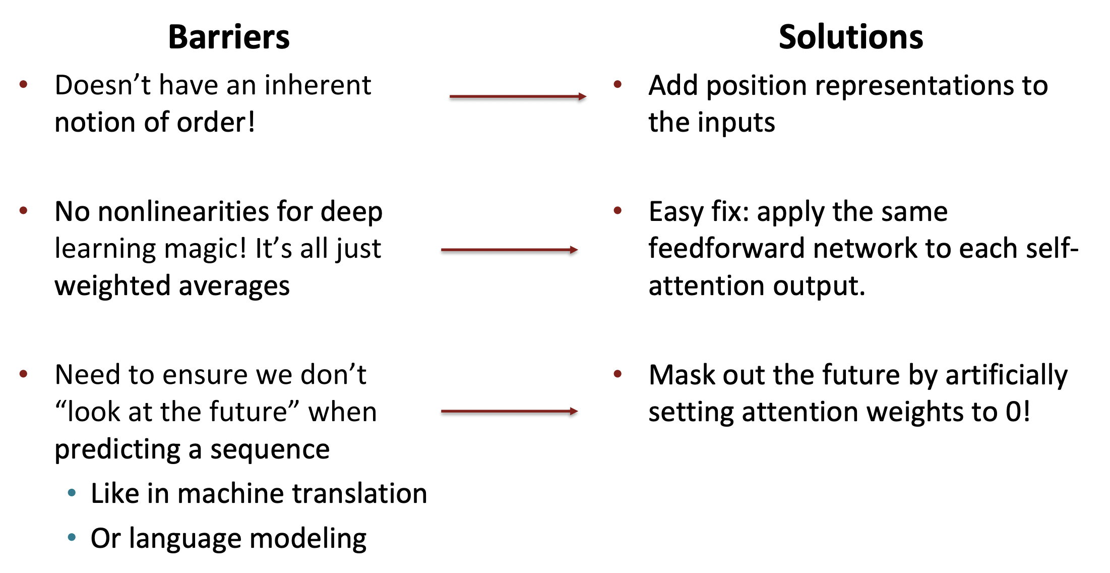
1️⃣ Self-attention doesn't know the order of its inputs.
💡 Add position representations to the inputs
-
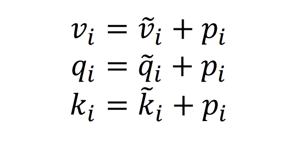
Self-attention이 순서 정보에 따라 build되지 않기 때문에 keys, queries, 그리고 values에서 sequence의 순서를 encode해야한다.
-
각 sequence index를 vector로 represent한다.

-
input(embedding vector)에 를 더한다.
- Deep self-attention에서, 이것은 첫번째 layer에서만 한다.
-
종류
- Sinusoidal position representations
- Learned absolute position representations
- Relative liner position attention
- Dependency syntax-based position
2️⃣ There are no elementwise nonlinearities in self-attention
💡 Adding nonlinearities in self-attention
- Feed-forward network를 추가하여 각 output vector를 post-process한다.
- = MLP() = * ReLU( * + ) +
- : output from self-attention
- Feed-forward network가 elementwise nonlinearity를 준다.
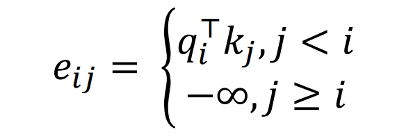
3️⃣ To use self-attention in decoders, we need to ensure we can't peek at the future
💡 Masking the future in self-attention
- Attention score을 −∞로 setting한다.
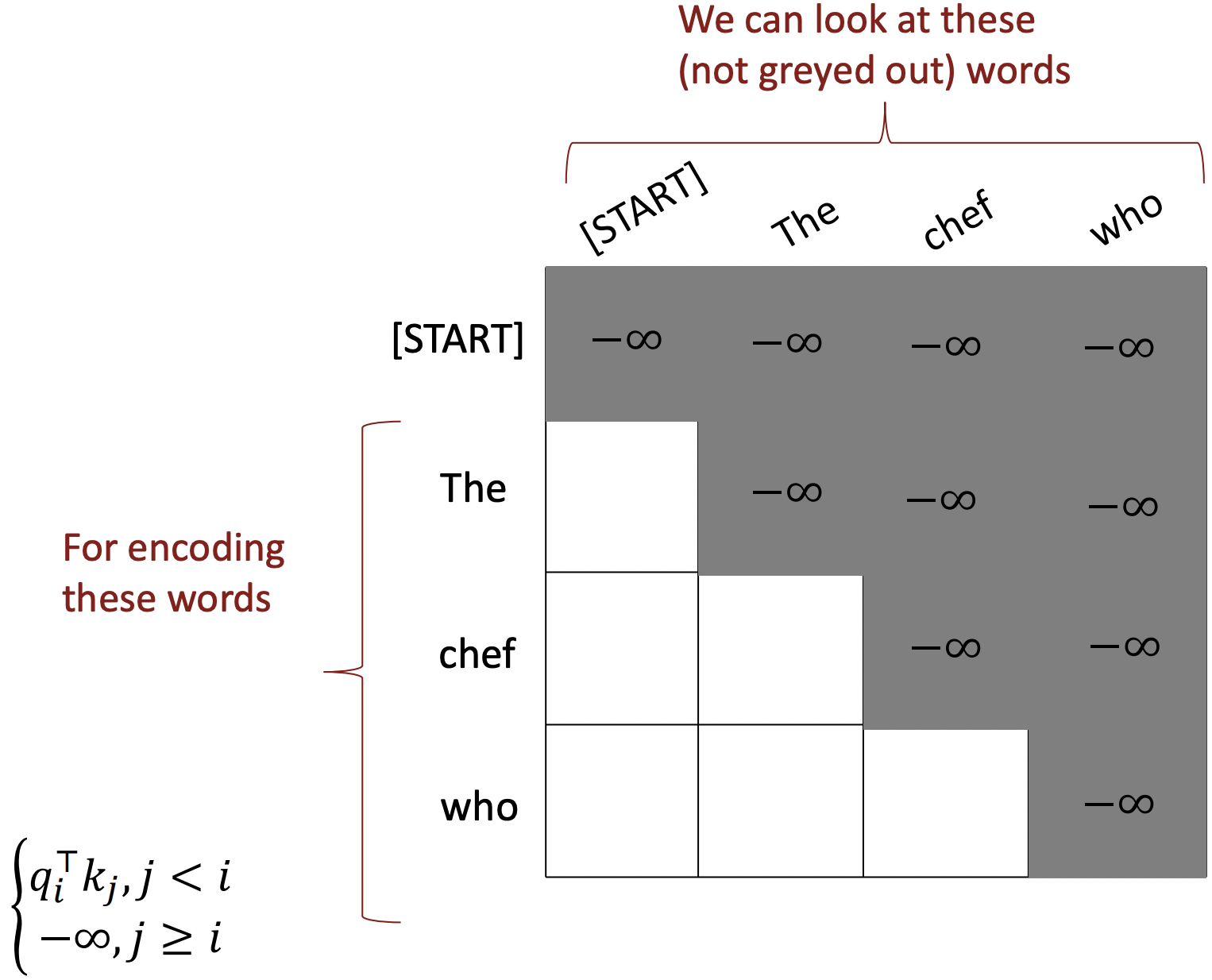
- Decoder의 모든 single layer에 이 masking이 필요하다.
✔️ Summary
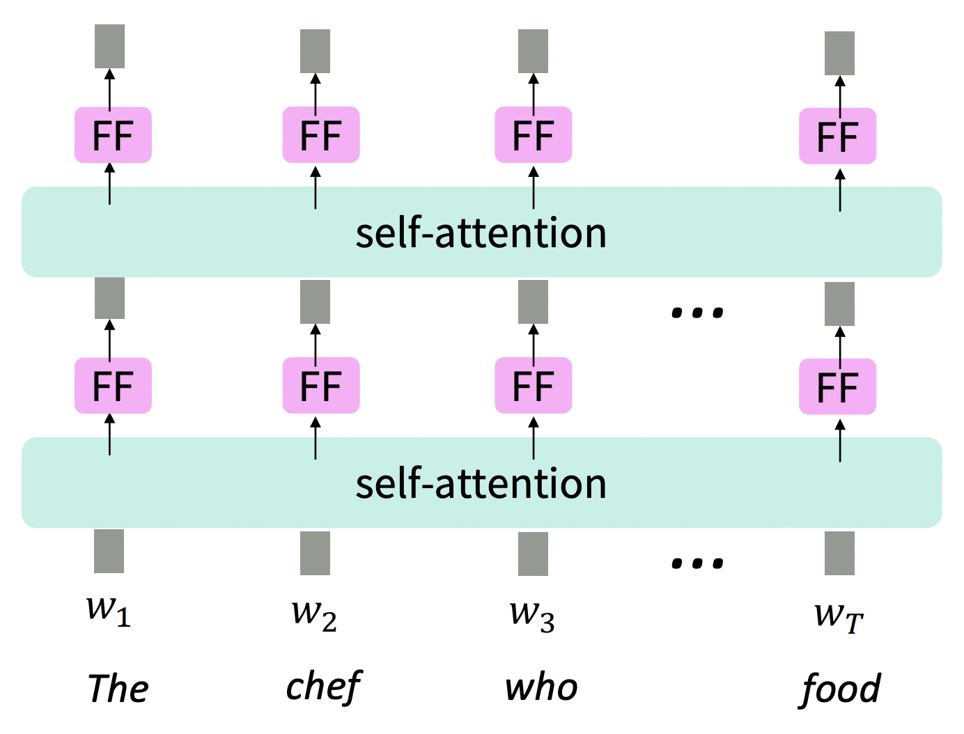
이제 Transformer Encoder-Decoder에 대해 알아보자.
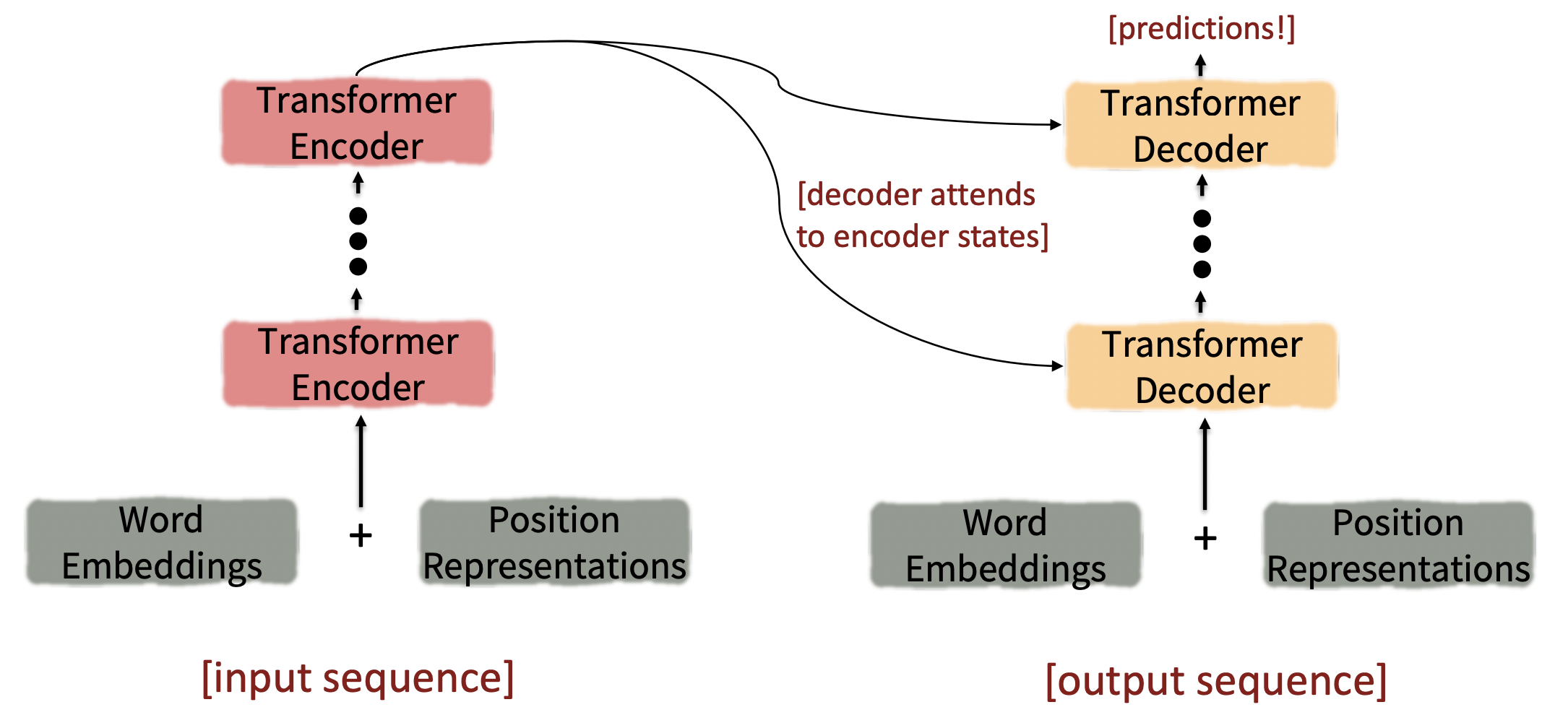
- Encoder의 마지막 layer가 각 decoder layer에 사용된다.
🔗 Transformer에서 중요한 세가지
- Key-query-value attention
- Multi-headed attention
- Tricks to help with training
- Residual connections
- Layer normalization
- Scaling the dot product
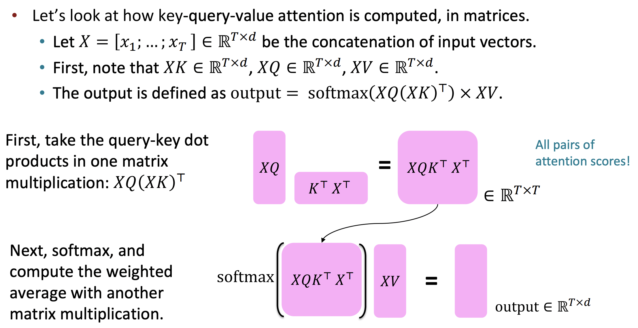
The transformer Encoder: Key-query-value attention
,...,를 Transformer encoder의 input vector라고 하자; ∈ R^d
- Each key = K, K ∈ R^d*d인 key matrix
- Each query = Q, Q ∈ R^d*d인 query matrix
- Each value = V, V ∈ R^d*d인 value matrix
- Dimensionality d에서 dimensionality d로 가는 transformation이다.
- Linear transformation을 적용했기 때문에 모든 k,g,v가 x와 같지 않고 살짝 다르다.
- 이 matrices를 통해 각 세 가지 역할에서 x의 각각 다른 측면을 강조/사용할 수 있다.
The transformer Encoder: Multi-headed attention
- Motivation : sentence에서 여러 곳에 attend하고 싶다.
- Multiple Q, K, V matrices를 통해 multiple attention "heads"를 정의한다.
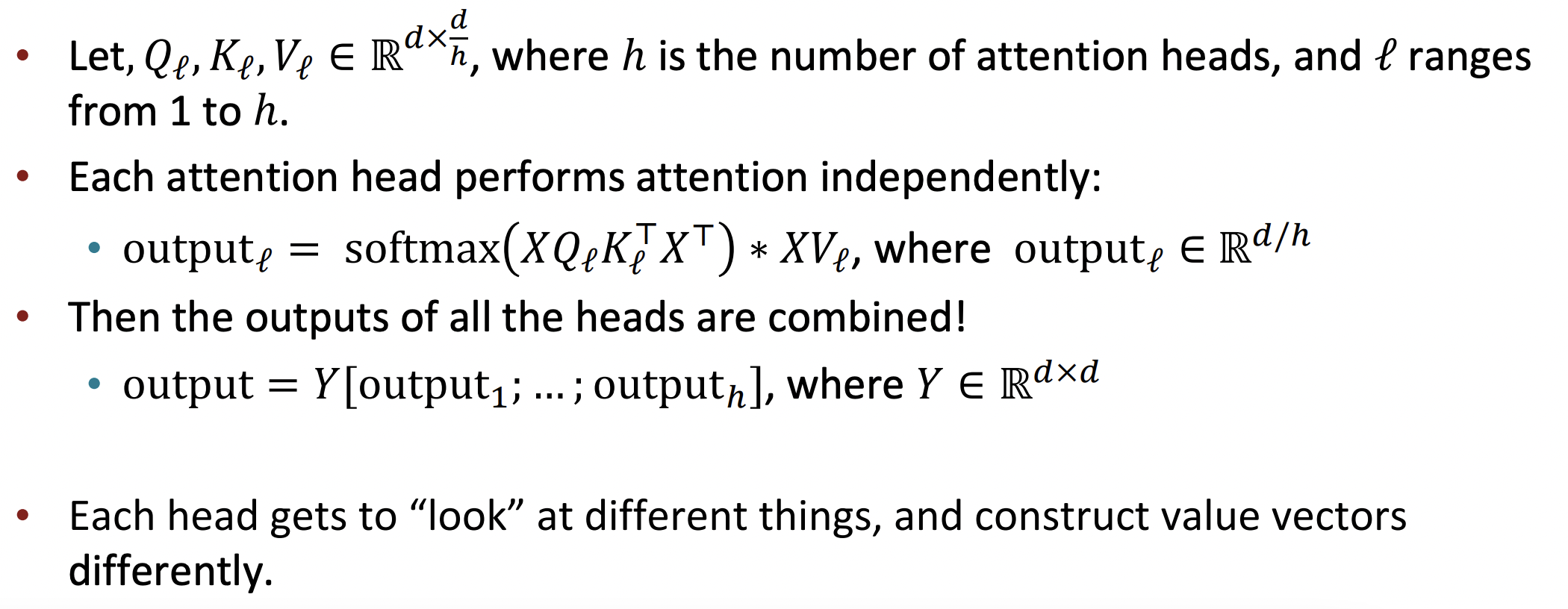
- 각 , , matrix들은 서로 다른 transformation을 학습한다.
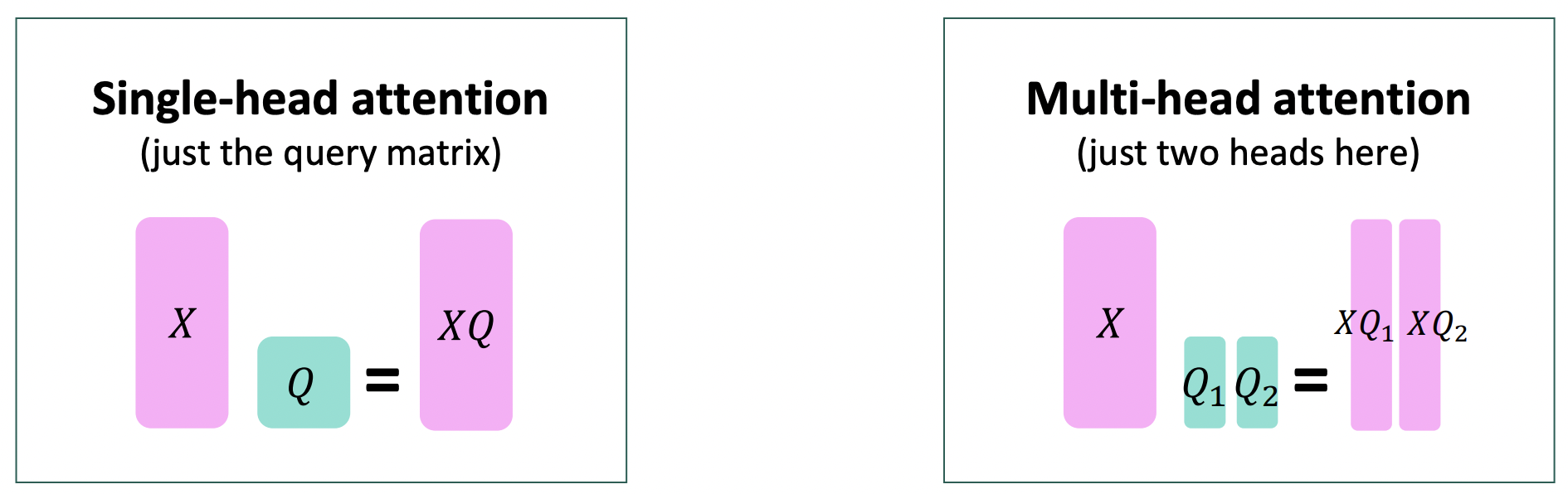
- Single-head self-attention과 Multi-headed self-attention의 연산량은 같다!
Tricks to help with training
🔗 The transformer Encoder: Residual connections
- X^(i) = X^(i-1) + Layer(X^(i-1))
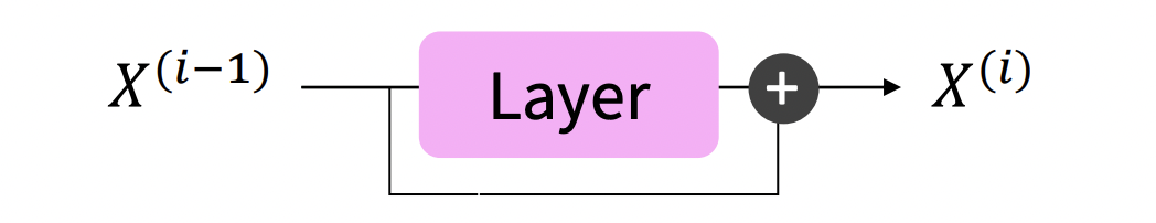
- Layer i가 Layer (i-1)과 어떻게 달라야 하는지 "the residual"을 배운다.
- Gradient 측면에서 보았을 때, 모든 것이 saturating 되어도 이 connection을 통해서 gradient가 전파된다.
- Residual connection은 loss landscape를 상당해 smoother하게 만들어 training이 더 쉬워지도록 한다.
🔗 The transformer Encoder: Layer normalization
- Idea : 각 layer 내에서 unit mean과 standard deviation으로 정규화하여 hidden vector values의 uninformative variation을 줄인다. 그리고 unit들이 서로 어떻게 다랐는지에 대한 informative variation은 유지된다.
- LayerNorm이 성공적인 이유는 아마 각 layer의 gradients를 normalize하기 때문일 것이다.
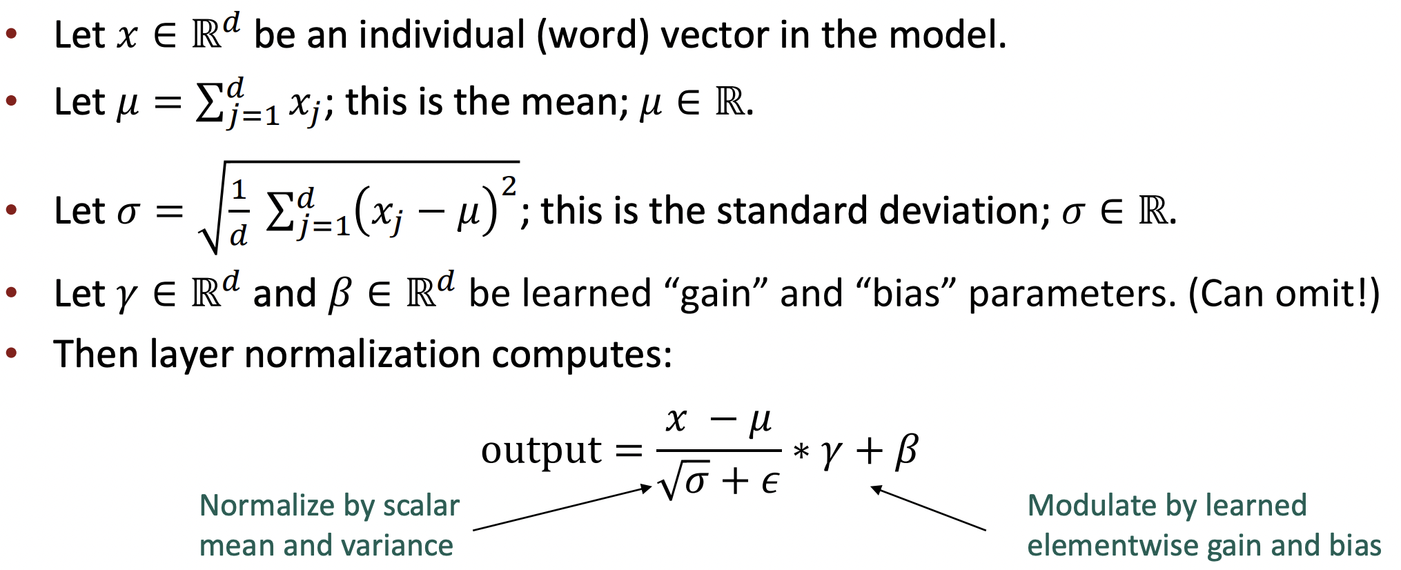
- 곱할 때는 hadamard product(elementwise multiplication) 사용
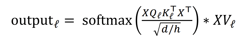
🔗 The transformer Encoder: Scaled Dot Product
-
Motivation : dimensionality d가 커지면, vector간의 dot product가 커지는 경향이 있다. 이렇게 dot product를 하면 variation이 커질텐데 그러면 softmax가 매우 peaky해질 수 있다. Attend되지 않는 connection은 거의 0에 가까워져 매우 낮은 probability distribution을 가지게 되고 gradient가 거의 없을 것이다.
-
Attention score를 (d/h)^1/2로 나누어 score가 커지는 것을 막는다.
The Transformer Decoder: Cross-attention
-
, ... , : output vectors from the Transformer encoder; ∈ R^d
-
, ... , : input vectors from the Transformer decoder; ∈ R^d
-
Keys와 values는 encoder에서 온다(메모리처럼).
- = K, = V
-
Queries는 decoder에서 온다.
- = Q
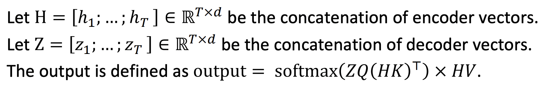
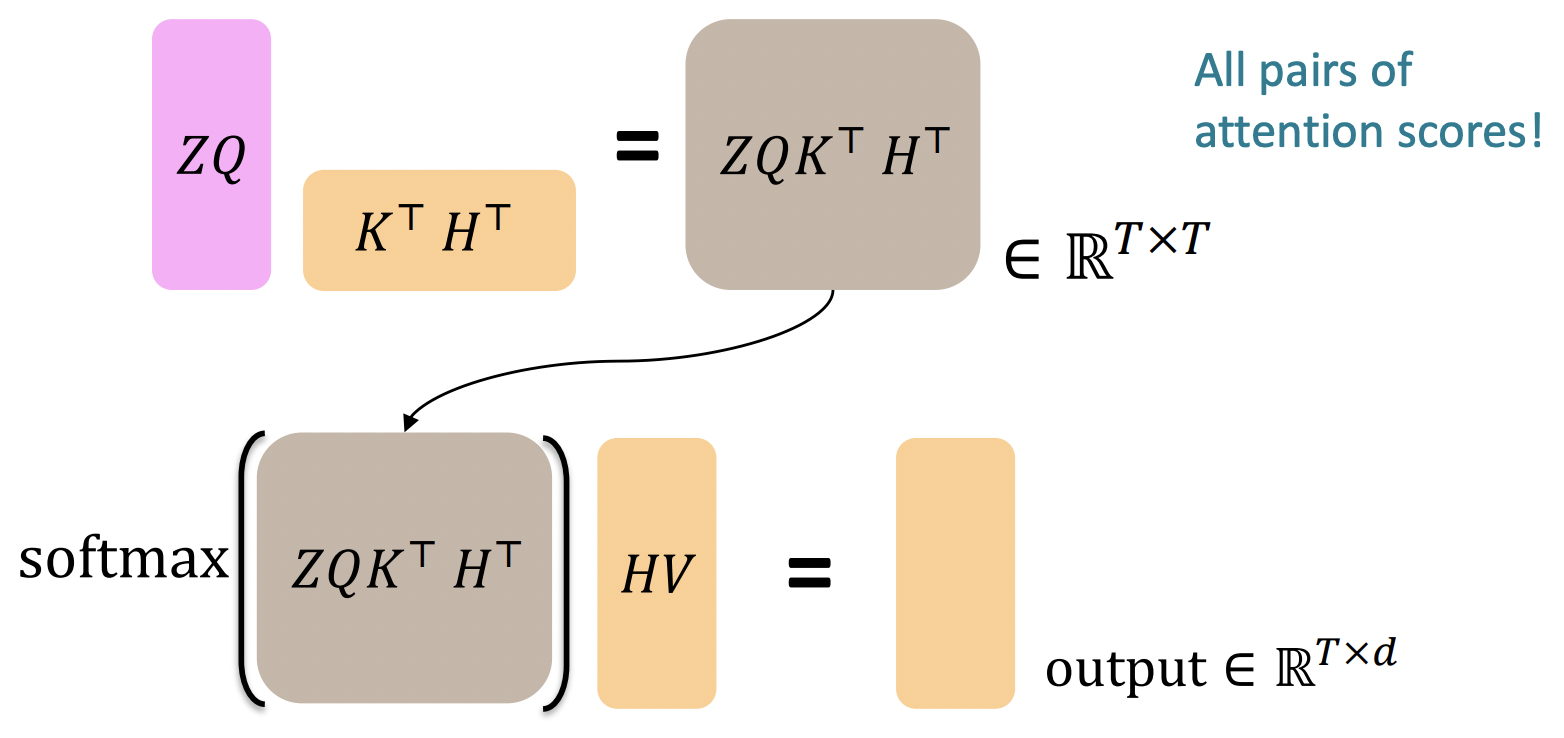
- output은 encoder에서 온 HV value vectors의 average이다. 그리고 average는 weights에 의해 결정된다.
Transformer Encoder-Decoder
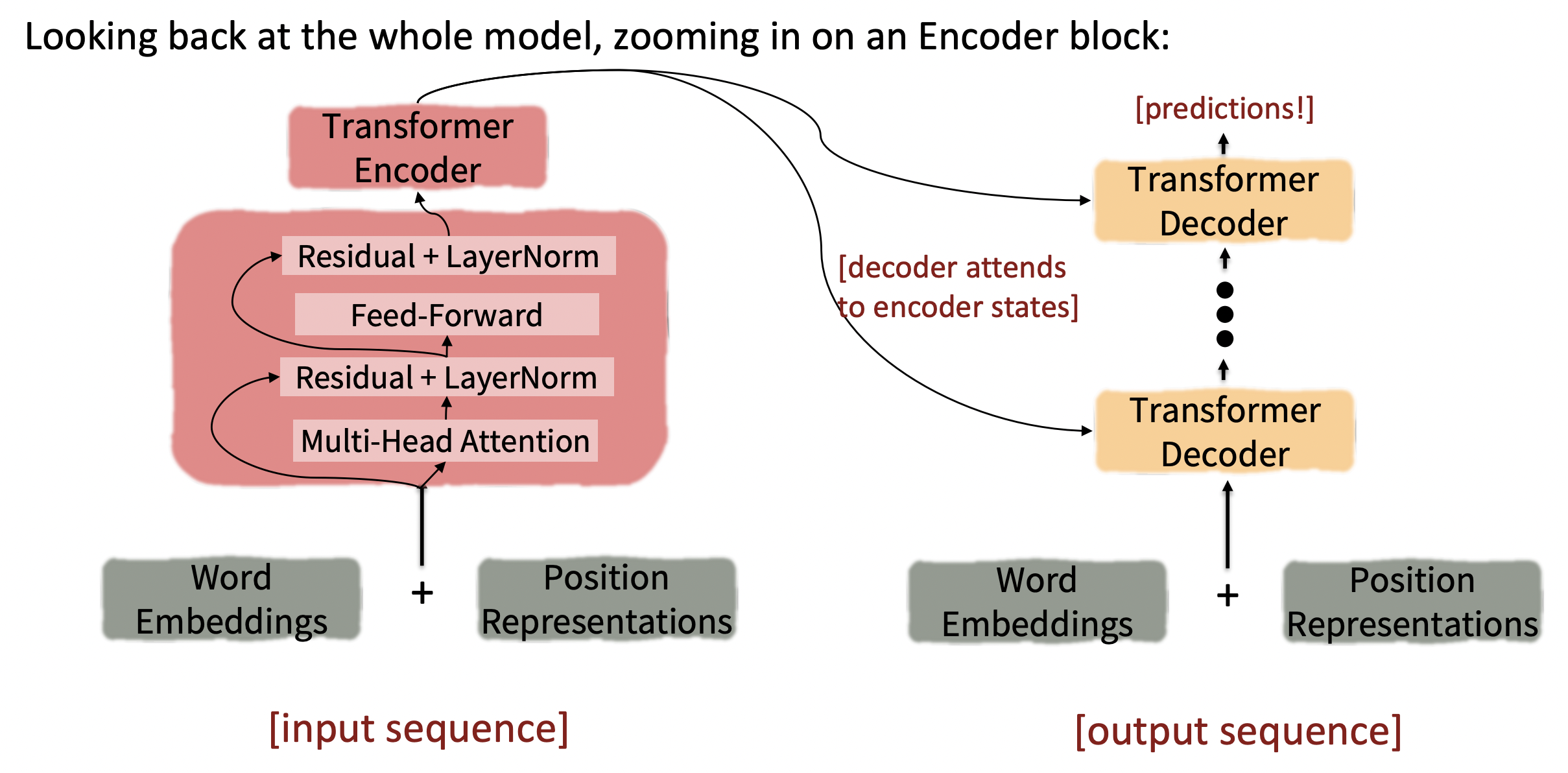
- Multi-Head Attention : Multi-head scaled dot product attention
- 마지막 Residual+LayerNorm의 output이 transformer encoder block의 output이다.
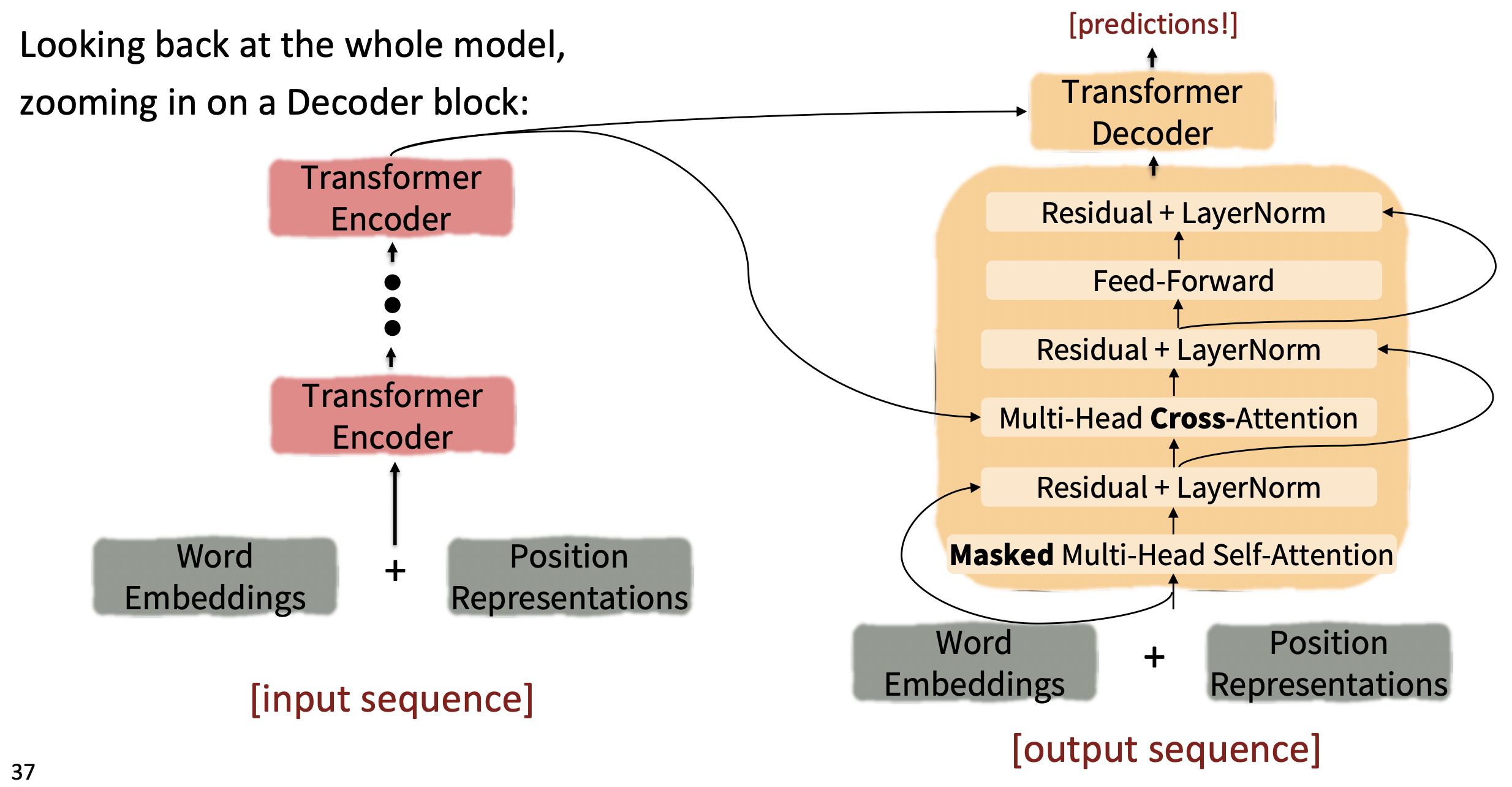
- Residual layer norm은 주목해야 할 것들 뒤에 항상 오는 것을 볼 수 있다. Residual layer norm은 gradients가 pass하도록 돕는다.
- 마지막 Residual+LayerNorm의 output이 transformer decoder block의 output이다.
Drawbacks of Transformers
🔗 Quadratic compute in self-attention
- 모든 interactions 쌍을 계산한다는 것은 연산량이 sequence length에 quadratically하게 증가한다는 것이다(T*T matrix).
- 반면에 recurrent model에서는 sequence length에 단지 linearly하게 자란다.
- Self-attention이 매우 parallelizable하다는 이점이 있지만, 전체 operation량이 는다는 것은 변함 없다.
- Total number of operations는 O(T^2d)로 자란다.
- T : sequence length
- d : dimensionality
🔗 Position representations
- Position(structure of sentence)을 represent할 수 있는 더 좋은 방법이 있을까?
Reference
- CS224n: Natural Language Processing with Deep Learning Lecture at Stanford University