선형회귀

---

기준모델(Baseline Model)

가장 간단한 최소한의 성능을 내는 모델

• 회귀 : 평균
• 분류 : 최빈값

x = df['sqft_living']
y = df['price']

baseline = y.mean()

sns.lineplot(x=x, y=baseline, color='red')
sns.scatterplot(x=x, y=y)
plt.show()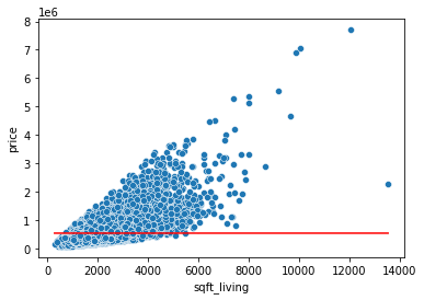

---

선형 회귀 모델

잔차제곱 합(RSS)을 최소화하는 직선

• 잔차(Residual) : 예측값과 관측값의 차이
• RSS(SSE) :
  ${\displaystyle \operatorname {RSS} =\sum _{i=1}^{n}(\varepsilon _{i})^{2}=\sum _{i=1}^{n}(y_{i}-f(x_{i}))^{2}=\sum _{i=1}^{n}(y_{i}-(\alpha x_{i} + \beta))^{2}}$

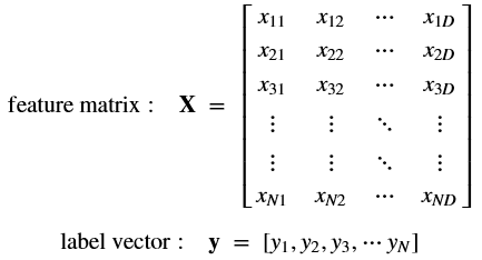
특성행렬 X : 2차원 행렬
타겟배열 y : 1차원 형태

방법1

#단순 선형 회귀 모델
model = LinearRegression() 

#모델 훈련
model.fit(X_train, y_train) 

X_test = [[x] for x in df_t['GrLivArea']] #2차원 데이터(특성행렬)
y_pred = model.predict(X_test) #test 데이터에 대한 회귀 예측

plt.scatter(X_train, y_train, color='black', linewidth=1) #train 데이터 
plt.scatter(X_test, y_pred, color='blue', linewidth=1); #test 예측 데이터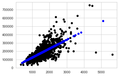

방법2

sns.regplot(x=df['GrLivArea'], y=['SalePrice'])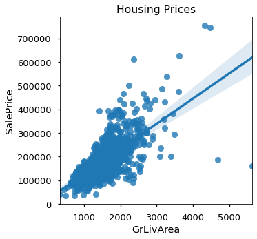

---

선형회귀모델 계수(Coefficients)

모델이 학습한 특성과 타겟의 관계

#계수, 절편
model.coef_, model.intercept_

(array([[107.13035897]]), array([18569.02585649])