다중 선형 회귀
다중 선형회귀 모델
- 2개 이상 특성의 선형회귀
그래프 확인
style.use('seaborn-talk')
fig = plt.figure()

ax = fig.gca(projection='3d')

x = 'GrlivArea'
y = 'OverallQual'
z = 'SalePrice'
ax.scatter(train[x], train[y], train[z]) #2개 특성과 1개 타겟의 3차원 scatter

plt.suptitle('Housing Prices')
plt.show()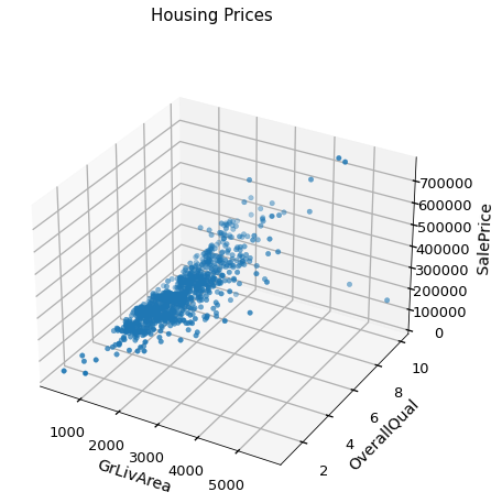
모델 학습
features = ['GrLivArea', 'OverallQual'] #2개 특성
X_train = train[features]
X_test = test[features]

model = LinearRegression()

model.fit(X_train, y_train)
y_pred = model.predict(X_train)
mae = mean_absolute_error(y_train, y_pred)
print(f'훈련 에러: {mae:.2f}')
훈련 에러: 29129.58
계수
model.intercept_, model.coef_(-102743.02342270731, array([ 54.40145532, 33059.44199506]))
회귀 모델 평가 지표
MAE
- 절대값 평균
MSE
- 제곱값 평균
RMSE
- MSE 제곱근
R-squared
- 결정계수
- 특성의 타겟 설명능력(0~1)
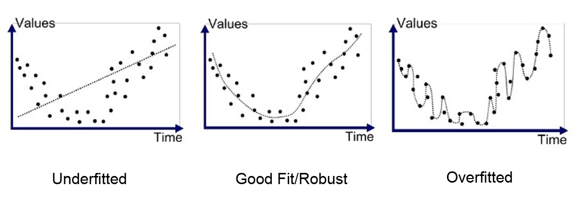
과적합, 과소적합
일반화
- 모든 데이터셋에서의 오차 정도
- val, test에서 좋은 성능을 내는 모델 = 일반화 잘된 모델
과적합
- 훈련 데이터의 정확도만 높은 상태
과소적합
- 모든 데이터의 정확도가 떨어지는 상태
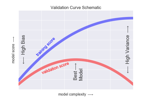
모델의 복잡도가 증가함에 따라 훈련데이터 성능은 증가하고 검증데이터 성능은 특정지점부터 감소
-> 과적합이 발생하는 시점
-> 학습 중지 필요
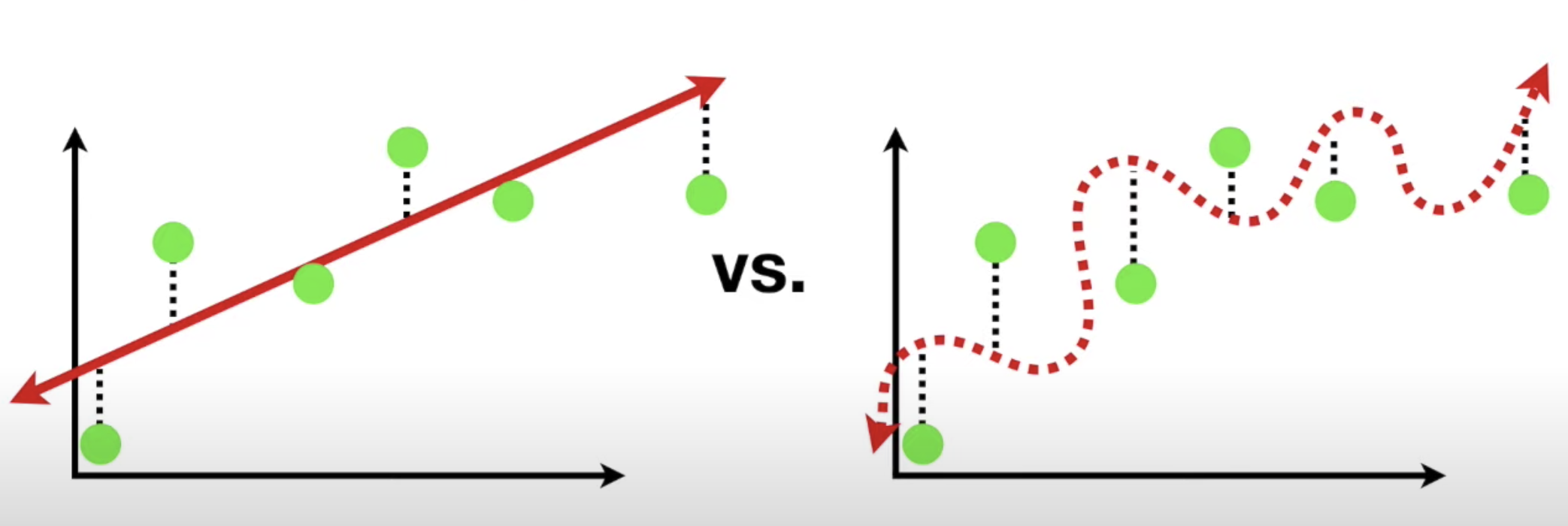
분산, 편향
분산
- 분산이 클 경우 과적합 상태(곡선)
편향
- 편향이 클 경우 과소적합 상태(직선)
다항 회귀
- 회귀계수의 차수가 2이상인 회귀 모델
#사용할 임시 데이터
rng = np.random.RandomState(1)
data = np.dot(rng.rand(2, 2), rng.randn(2, 30)).T
X = pd.DataFrame([i[0] for i in data])
y = pd.DataFrame([i[1] for i in data])

X_train, X_test, y_train, y_test = train_test_split(X, y, random_state=1)

#다항 회귀 차수 지정
model = PolynomialRegression(3)

model.fit(X_train, y_train)

plt.scatter(X_train, y_train, color='blue', alpha=0.5)
plt.scatter(X_test, y_test, color='red', alpha=0.5)

x_domain = np.linspace(X.min(), X.max()) #예측 범위
curve = model.predict(x_domain)
plt.plot(x_domain, curve, color='blue')
plt.show()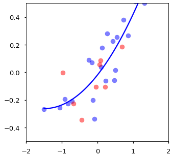
#6차항
model = PolynomialRegression(6) 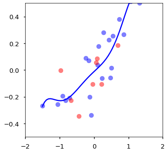
#10차항
model = PolynomialRegression(10) 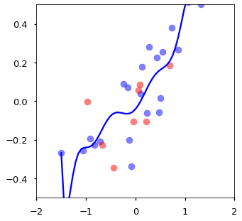

모치