
부트캠프 프로젝트 정리용
목차
1. EDA
- 매출 데이터 정리(K, M 제거)
- 연도 데이터 수정(형식 변경, 결측치 기입)
2. Popular Game Genre by Region
- 지역별 장르 매출 합산
3. Popular Game Genre by Year
- 연도별 장르 매출 합산
- 필요한 기간의 데이터 선정하여 그래프 plot
4. Sales Similarity by Genre
- 지역별 장르 매출의 PCA 진행
- 최적의 K값 선정
- PCA 결과 기반 Clustering
1. EDA
1. 데이터 호출하여 데이터 확인
import pandas as pd
df = pd.read_csv('vgames2.csv')
df.head()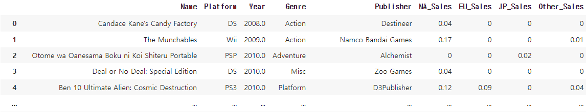
2. 불필요 데이터 제거
Unnamed: 0, 중복데이터
df.drop('Unnamed: 0', axis=1, inplace=True)
df.drop_duplicates(inplace=True)
df.shape
3. 매출 데이터 K,M 문자 제거
df_list = []

# K,M 포함 매출 데이터 수정
# M을 기본 단위로
for i in range(df.loc[:,'NA_Sales':'Other_Sales'].shape[1]):
  j = i+5

  # K,M 포함 행 추출
  df_k = df[df.iloc[:,j].str.contains('K') == True].copy()
  df_m = df[df.iloc[:,j].str.contains('M') == True].copy()

  # K포함 행은 K삭제 후 1000나누기, M포함 행은 M삭제만 진행
  df_k.iloc[:,j] = df_k.iloc[:,j].str.extract('(\d+)').astype(float)/1000
  df_m.iloc[:,j] = df_m.iloc[:,j].str.extract('(\d+)').astype(float)

  # 정리한 행 합치기
  df_c = pd.concat([df_k, df_m])
  df_list.append(df_c.iloc[:,j])

df_num = pd.concat(df_list, axis=1)
df_num.head()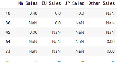
# 수정한 매출 데이터 덮어쓰기
df.update(df_num, overwrite=True)


# float으로 변경
df.iloc[:,5:9] = df.iloc[:,5:9].astype(float)
df.info()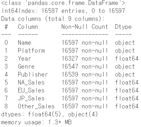
4. 연도 이상 데이터 수정
xx형식 -> 20xx 으로 수정이상치 직접 수정
# 연도수정 - 1
# 30미만은 19oo, 30이상 100미만은 20oo
df_year_30 = df.query('Year < 30').copy()
df_year_100 = df.query('(Year >= 30) & (Year < 100)').copy()

df_year_30['Year'] = df_year_30['Year'] + 2000
df_year_100['Year'] = df_year_100['Year'] + 1900

df_year_00 = pd.concat([df_year_30, df_year_100], axis=0)
df_year_00

# 데이터 업데이트
df.update(df_year_00, overwrite=True)
df_year = df.sort_values('Year').reset_index(drop=True)
df_year.head()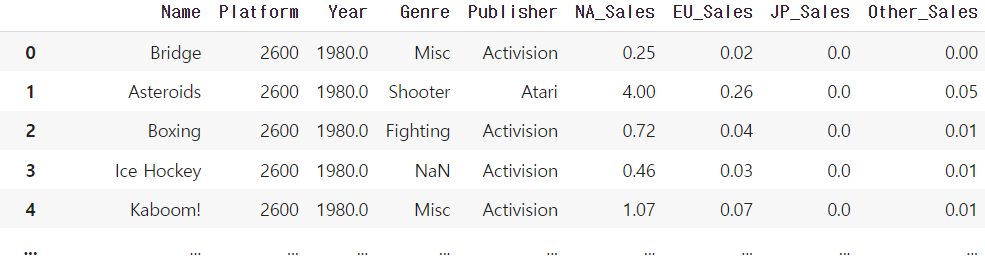
# 연도수정 - 2
df.loc[6906, 'Year'] = 2009.0
df.loc[10107, 'Year'] = 2016.0
df.loc[15233, 'Year'] = 2016.0
df.loc[5310, 'Year'] = 2016.0

df[df['Name'].str.contains('Imagine: Makeup Artist')] #데이터 수정 확인
6. 연도 결측치 기입
이름별로 묶어 평균치 기입연도 결측치 제거
# 그룹의 평균 연도로 결측치 수정
fill_func = lambda g: g.fillna(g.mean())
df_year_num = df.iloc[:,:3].groupby('Name').apply(fill_func) #그룹별로 함수 적용

# 결측치 입력한 데이터프레임 이름순서 정렬
df_year_num.reset_index(drop=True, inplace=True)
df_year_num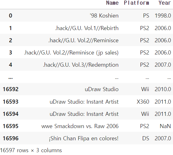
# 기존 데이터프레임 이름순서 정렬
df = df.sort_values('Name').reset_index(drop=True)

# 위 두 데이터로 업데이트
df.update(df_year_num, overwrite=True)
7. 결측치 중 평균 이상매출을 가지는 연도 데이터는 직접 기입
# 연도 결측치 데이터 추출
df_year_na = df[df['Year'].isna()].loc[:,['Name', 'Platform', 'NA_Sales', 'EU_Sales', 'JP_Sales', 'Other_Sales']].reset_index()
df_year_na = df_year_na.groupby(['index']).sum().sum(axis=1).sort_values(ascending=False)

# 평균이상 데이터의 결측연도 기입
df_year_mean = pd.DataFrame(df_year_na[df_year_na > df_year_na.mean()])

df_year_mean['Year'] = [2005, 2007, 2001, 2007, 2007, 1998, 1980, 1977, 2007, 1999, 1997, 2002, 1977, 2010, 2004, 2011, 2011,
                      2008, 2006, 1980, 1982, 1980, 2008, 2008, 1978, 1978, 2010, 2011, 2002, 2001, 2008, 2002, 1978, 2006,
                      2004, 1980, 2004, 1979, 2000, 2008]

df_year_mean = df_year_mean['Year'].astype(float)

df.update(df_year_mean, overwrite=True)
df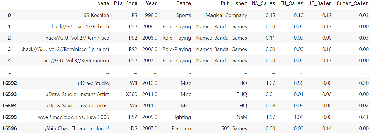
2. Popular Game Genre by Region
1. 지역별 장르 매출 합산
# 매출 columns 추출
df_sales = df.loc[:,['Genre','NA_Sales', 'EU_Sales', 'JP_Sales', 'Other_Sales']]

# 지역의 장르별 매출 합계
df_sales = df_sales.groupby('Genre').sum()
df_sales_ind = df_sales.reset_index()
df_sales_ind.set_index('Genre')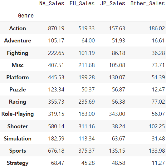
2. 4개 지역의 장르별 매출 plot
import seaborn as sns
import matplotlib.pyplot as plt

# 전체 그래프 크기 지정
fig = plt.figure()
fig.set_figheight(df_sales.shape[1]*4)
fig.set_figwidth(10)

# 4개지역 바그래프
for i in range(df_sales.shape[1]):
  plt.subplot(df_sales.shape[1], 1, i+1)
  sns.barplot(x='Genre', y=df_sales_ind.iloc[:,i+1], data=df_sales_ind)
  plt.ylim(0, 1000);
  plt.xticks(rotation=35); #x축 눈금 레이블 회전

fig.tight_layout() #겹침방지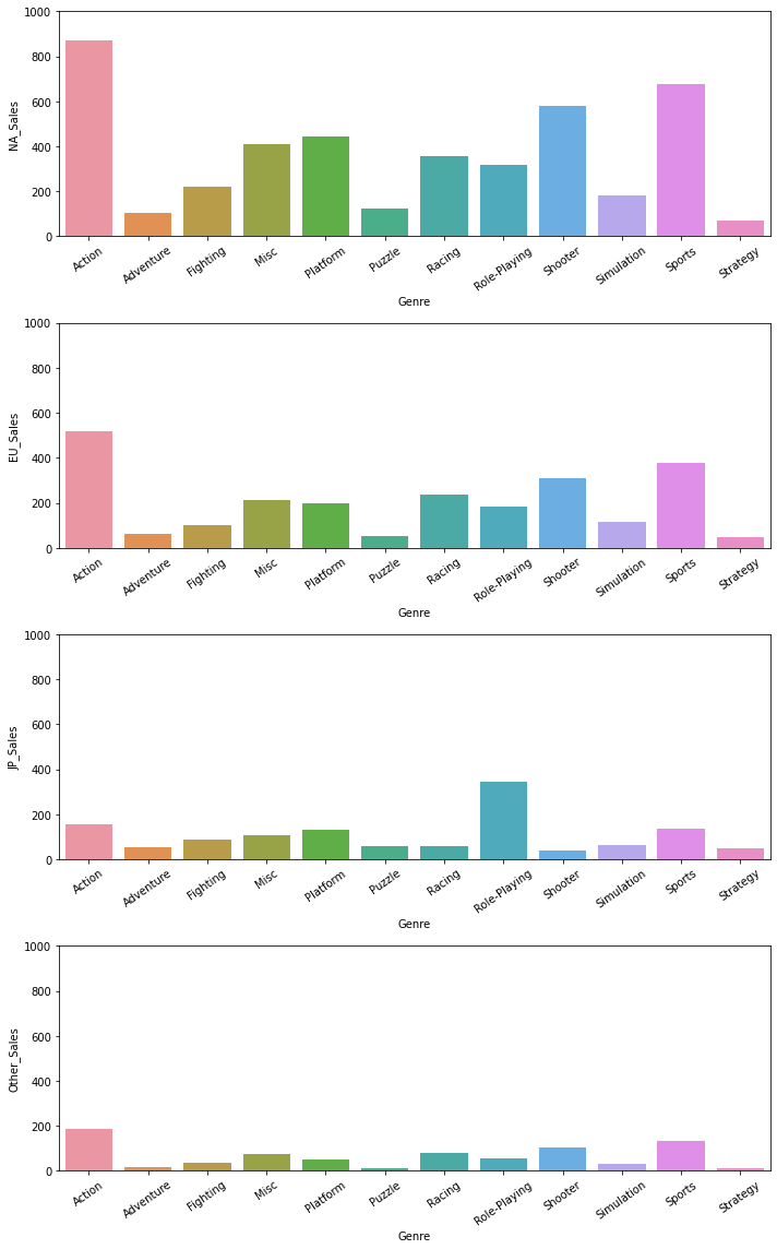
3. Popular Game Genre by Year
1. 연도별 장르 매출 합산
# 연도 결측치 제거, 정수형 변환
df_year_drop = df.dropna(subset=['Year']).copy()
df_year_drop['Year'] = df_year_drop['Year'].astype(int)
# Genre와 Year 기준 합산
df_group = df_year_drop.groupby(['Genre', 'Year']).sum().sum(axis=1)
df_group = df_group.unstack()
df_group_ind = df_group.reset_index()
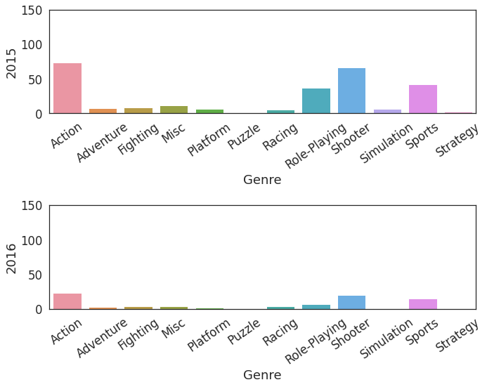
df_group_ind.set_index('Genre')2. 전체기간 연도별 막대그래프 plot
fig = plt.figure()
fig.set_figheight(df_group.shape[1] * 4)
fig.set_figwidth(10)

# 연도별 장르 매출 추이
for i in range(df_group.shape[1]):
  plt.subplot(df_group.shape[1], 1, i+1)
  sns.barplot(x='Genre', y=df_group_ind.iloc[:,i+1], data=df_group_ind)
  plt.ylim(0, 150);
  plt.xticks(rotation=35);

fig.tight_layout()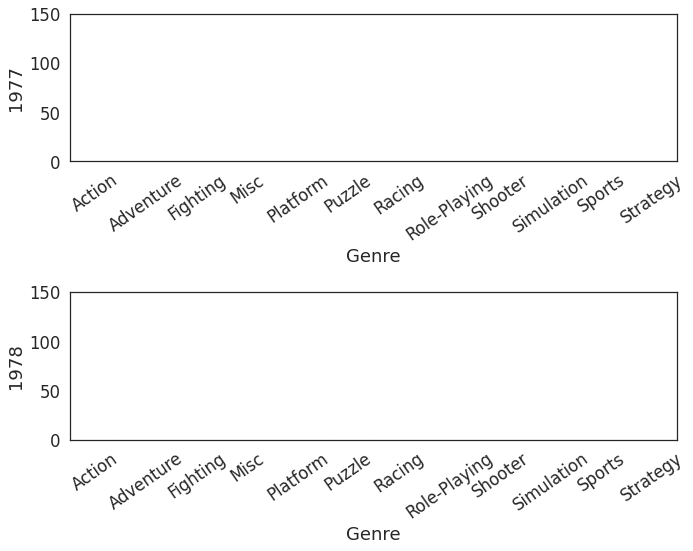
...
...
3. 매출 합산 그래프 plot
fig = plt.figure()
fig.set_figheight(8)
fig.set_figwidth(13)

for i in range(df_group_ind.shape[0]):
  data = df_group_ind.iloc[i,1:]
  plt.plot(data, label=df_group_ind.iloc[i,0]);
  plt.xlim(1976, 2017);
plt.legend();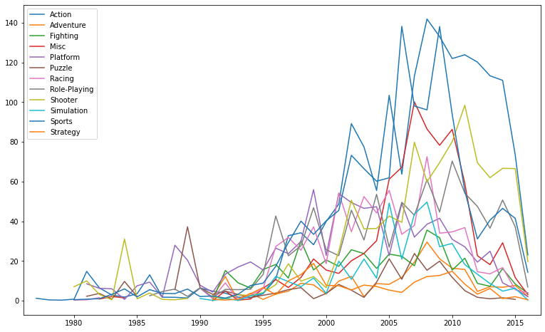
4. 데이터가 부족한 2016년 column 삭제
fig = plt.figure()
fig.set_figheight(8)
fig.set_figwidth(13)

# 16년 데이터 삭제한 데이터 생성
df_group_ind15 = df_group_ind.iloc[:,:-1]

# 삭제한 후 그래프 plot
for i in range(df_group_ind15.shape[0]):
  data = df_group_ind15.iloc[i,1:]
  plt.plot(data, label=df_group_ind15.iloc[i,0]);
  plt.xlim(1976, 2017);
plt.legend();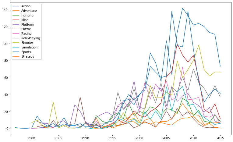
5. 연도별로 장르 매출 내림차순 정리하여 합치기
# 연도별 순위 메기기
rank_list = []
for i in range(df_group_ind15.shape[1]-1):
  j=i+1
  # 연도별 매출 순위 추출
  df_rank_com = df_group_ind15[['Genre', df_group_ind15.columns[j]]].dropna().sort_values(df_group_ind15.columns[j], ascending=False).reset_index(drop=True)

  # 순위 데이터 담은 리스트 제작
  rank_list.append(df_rank_com)

df_rank = pd.concat(rank_list, axis=1)
df_rank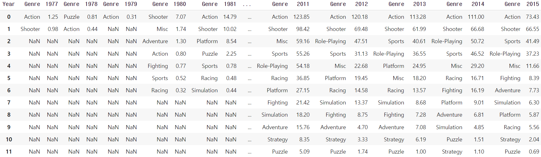
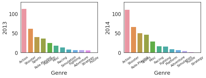
6. 연도별 순위 바그래프 plot
fig = plt.figure()
fig.set_figheight((df_rank.shape[1]/2) * 4)
fig.set_figwidth(10)

# 연도별 인기 장르 추이
for i in range(int(df_rank.shape[1]/2)):
  plt.subplot(df_rank.shape[1]/2, 2, i+1)
  sns.barplot(x=df_rank.iloc[:,i*2], y=df_rank.iloc[:,(i*2)+1], data=df_rank)
  plt.ylim(0, 130);
  plt.xticks(rotation=35);

fig.tight_layout()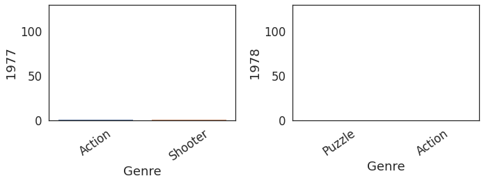
...
...
4. Sales Similarity by Genre
1. (2-1.)지역별 장르 매출 합산
#df_sales2. 장르들간의 PCA 진행
2개의 PC 선정
import numpy as np
from sklearn.preprocessing import StandardScaler
from sklearn.decomposition import PCA

scaler = StandardScaler()
pca = PCA()

# 데이터 표준화
Z = scaler.fit_transform(df_sales)

# pca 적용
B = pca.fit_transform(Z)
df_b = pd.DataFrame(B)
df_b.columns = ['pc1', 'pc2',' pc3', 'pc4']

# pca 비율 확인
pca.explained_variance_ratio_
3. 장르별로 매출 특성이 위치하는 산점도 plot
# 장르와 pc1, pc2 columns 합치기
gen = df_sales.reset_index().iloc[:,0]
df_new = pd.concat((df_b[['pc1', 'pc2']], gen), axis=1)

# 장르별로 pc 2차원 평면에 산점도 plot
sns.set(font_scale=1.5)
sns.set_style('white')
ax = sns.lmplot(x='pc1', y='pc2', data=df_new, hue='Genre', fit_reg=False)
ax.fig.set_size_inches(16, 8)

fig.tight_layout()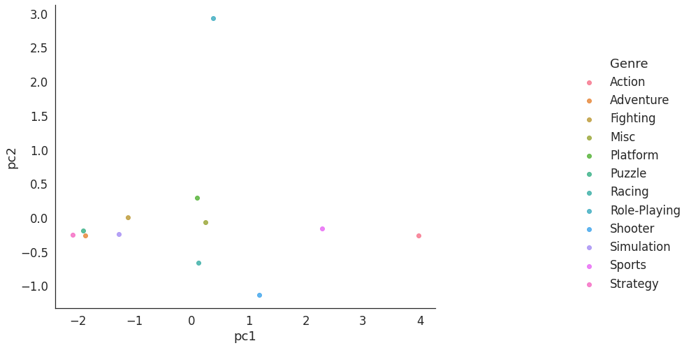
4. 최적의 k값 선정(elbow method)
sse = {}
for k in range(1, 10):
  kmeans = KMeans(n_clusters = k, random_state=42)
  kmeans.fit(df_new.iloc[:, :2])
  sse[k] = kmeans.inertia_

plt.title('title')
plt.xlabel('x')
plt.ylabel('y')
sns.pointplot(x=list(sse.keys()), y=list(sse.values()));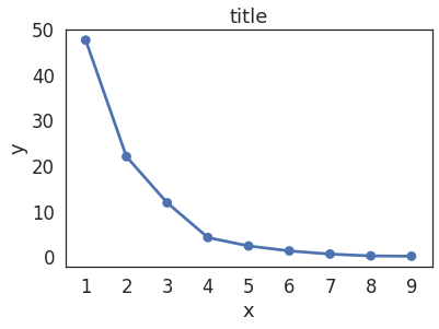
4. PCA 결과 기반 Clustering 산포도 plot
from sklearn.cluster import KMeans

# k = 4
kmeans = KMeans(n_clusters = 4, random_state=42)
kmeans.fit(df_new.iloc[:,:2])
cluster_labels = kmeans.labels_
print(kmeans.inertia_)

# cluster 라벨 붙임
df_new['cluster'] = cluster_labels

# cluster 기반 산포도
sns.set(font_scale=1.5)
sns.set_style('white')
ax = sns.lmplot(x='pc1', y='pc2', data=df_new, hue='cluster', fit_reg=False)
ax.fig.set_size_inches(14, 9)
fig.tight_layout()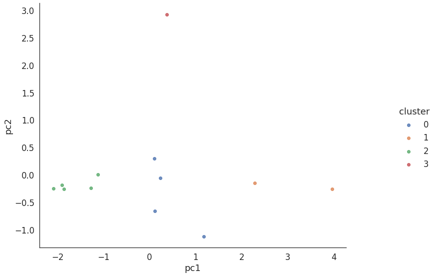
결론
- 최고 매출 지역 : 미국
- 미국 내 최고 매출 장르 : 액션
- 최근 5년 매출 상위 장르 : 액션, 슈팅, 스포츠
- 액션과 유사한 매출의 장르 : 스포츠

모치