[AI/ML] 파이썬 머신러닝 완벽가이드 (4) - cross_val_score(), GridSearchCV

cross_val_score()

앞에서 K Fold, Stratified K Fold 이용하여 데이터들로 Decision Tree Classifier 모델을 학습시키고 교차검증하는 과정을 거쳤다. K Fold 혹은 Stratified K Fold 객체의 split 메소드를 사용하여 교차검증에 사용할 인덱스로 만들어진 어레이를 이터레이션 돌아갈 수 있게 먼저 만들어준다.

(array([2, 3, 4, 5, 6, 7, 8, 9]), array([0, 1]))  # 첫 번째 반복
(array([0, 1, 4, 5, 6, 7, 8, 9]), array([2, 3]))  # 두 번째 반복
(array([0, 1, 2, 3, 6, 7, 8, 9]), array([4, 5]))  # 세 번째 반복
(array([0, 1, 2, 3, 4, 5, 8, 9]), array([6, 7]))  # 네 번째 반복
(array([0, 1, 2, 3, 4, 5, 6, 7]), array([8, 9]))  # 다섯 번째 반복

그리고 이렇게 얻어낸 인덱스를 이용해서 학습 데이터와 테스트 데이터를 나누고 학습 및 평가를 진행한다.

# Stratified K Fold
import pandas as pd
import numpy as np
from sklearn.model_selection import StratifiedKFold
from sklearn.datasets import load_iris
from sklearn.tree import DecisionTreeClassifier
from sklearn.metrics import accuracy_score

iris = load_iris()
features=iris.data
label=iris.target
iris_df = pd.DataFrame(data=iris.data, columns=iris.feature_names)
iris_df['label'] = iris.target
print(iris_df['label'].value_counts())
dt_clf=DecisionTreeClassifier(random_state=156)

# StratifiedKFold 객체 생성
skfold = StratifiedKFold(n_splits=3)
n_iter = 0
cv_accuracy=[]

# StratifiedKFold의 split() 호출시 반드시 레이블 데이터 셋도 추가 입력 필요.
for train_index, test_index in skfold.split(iris_df, iris_df['label']):
    n_iter += 1
    X_train, X_test= features[train_index], features[test_index]
    y_train, y_test= label[train_index], label[test_index]
    label_train = iris_df['label'].iloc[train_index]
    label_test = iris_df['label'].iloc[test_index]
    # print(f'#{n_iter} train index: {train_index}')
    # print(f'#{n_iter} test index: {test_index}')
    print(f'## 교차 검증: {n_iter}')
    print(f'학습 레이블 데이터 분포:\n{label_train.value_counts()}')
    print(f'검증 레이블 데이터 분포:\n{label_test.value_counts()}')
    dt_clf.fit(X_train, y_train) # 모델 학습
    pred = dt_clf.predict(X_test) # 예측
    accuracy = np.round(accuracy_score(y_test, pred)) # 정확도 측정
    cv_accuracy.append(accuracy)
    
    print(f'#{n_iter} 교차 검증 정확도: {accuracy}, 학습 데이터 크기: {X_train.shape[0]}, 검증 데이터 크기: {X_test.shape[0]}')
    
print(f'## 교차 검증별 정확도: {cv_accuracy}')

Stratified K Fold를 이용하는 코드.

그런데 이 과정에서 split() 메소드로 나누고, 학습 및 테스트데이터 설정, 학습, 테스트, 검증에 쓰이는 코드가 좀 길게 느껴져 이걸 사이킷런에서 한 묶음으로 cross_val_score()라는 메소드로 간편히 사용할 수 있게 만들어놓았다. 이를 이용하면 for loop 돌 필요 없이 코드를 줄일 수 있다. cross_val_score()는 기본적으로 stratified k fold 방법으로 데이터를 분리한다.

import numpy as np
import pandas as pd
from sklearn.datasets import load_iris
from sklearn.tree import DecisionTreeClassifier
from sklearn.metrics import accuracy_score
from sklearn.model_selection import cross_val_score

# 데이터 불러오기
iris = load_iris(as_frame=True) # DataFrame으로 불러오기.
iris_data_df= iris.data
iris_label = iris.target

# 학습모델 객체 생성
dt_clf = DecisionTreeClassifier(random_state=156)

# cross_val_score 이용해서 k=3인 stratified k fold로 교차검증.
cv_accuracy = cross_val_score(dt_clf, iris_data_df, iris_label, scoring='accuracy', cv=3)
print(f'교차 검증별 정확도: {cv_accuracy}')

cross_val_score() 메소드를 사용하는 코드. 확실히 양이 줄어든다.

메소드의 각 패러미터에 대한 내용은 다음과 같다.

dt_clf: 학습모델 객체
iris_data_df: Feature 데이터
iris_label: Label 데이터
scoring='accuracy': 정확도 측정
cv=3: 3개의 폴드 세트로 분리하는 KFold로 교차검증 수행.

코드를 수행하면 cross_val_score()통해 각 교차검증별 정확도 정보가 ndarray 형으로 반환된다. 이를 가지고 np.mean() 으로 평균을 내주면 전체 교차검증의 평균정확도를 알 수 있다.

GridSearchCV

GridSearchCV란, 모델의 성능을 더 고도화하기 위해 사용하는 기법 중 하나로, 하이퍼 파라미터 값들을 격자 형태로 쪼개어 최적의 하이퍼 파라미터 값을 찾아가는 방식을 말한다. 만약 파라미터1에서 4개의 경우와 파라미터 2에서 4개의 경우를 튜닝하고 싶다면 총 4x4=16 번의 학습결과를 보면서 최적의 파라미터를 찾아나가게 된다. 이렇듯 격자를 하나하나 돌면서 모델을 학습시키다보니 튜닝하고자 하는 값이 많으면 오래걸린다는 단점이 있다. 여기서 하이퍼 파라미터는 모델이랑은 직접적인 관련이 없지만 학습을 좀 더 잘할 수 있도록 도와주는 파라미터를 말한다.

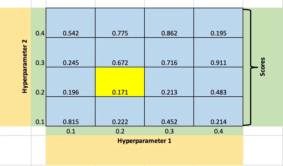
하이퍼 파라미터 1, 2 각각에 따른 모델의 평가점수

iris 데이터에서 max_depth 와 min_samples_split 을 변경해가며 수행하여 최적 하이퍼 파라미터가 어떤 경우인지 찾아보자.

# GridSearchCV

import numpy as np
import pandas as pd
from sklearn.datasets import load_iris
from sklearn.tree import DecisionTreeClassifier
from sklearn.metrics import accuracy_score
from sklearn.model_selection import train_test_split, GridSearchCV

# 데이터 준비. DataFrame 형으로.
iris = load_iris(as_frame=True)
iris_data_df = iris.data
iris_label=iris.target

# train data와 test data로 분리.
X_train, X_test, y_train, y_test = train_test_split(iris_data_df, iris_label, test_size=0.2, random_state=11)

# parameter들을 dictionary 형태로 설정.
parameters = {'max_depth':[1,2,3],'min_samples_split':[2,3]}


# params_grid의 하이퍼 패러미터들을 3개의 train, test set fold로 나누어 테스트 수행 설정.
# refit=True 가 기본값. True면 가장 좋은 패러미터 설정으로 재학습시킴.
# GridSearchCV
dt_clf=DecisionTreeClassifier(random_state=156)
grid_dtree=GridSearchCV(estimator=dt_clf, param_grid=parameters, cv=3, refit=True, return_train_score=True)

# 붓꽃 train 데이터로 param_grid의 하이퍼 패러미터를 순차적으로 학습/평가.
grid_dtree.fit(X_train, y_train)

# GridSearchCV 결과는 학습된모델.cv_results_ 라는 딕셔너리로 저장 됨.
cv_results_df= pd.DataFrame(grid_dtree.cv_results_)
display(cv_results_df)

# 최적 파라미터는 학습된모델.best_params_, 최고 정확도는 학습된모델.best_score_
print(f'최적 파라미터: {grid_dtree.best_params_}')
print(f'최고 정확도: {grid_dtree.best_score_}')

# refit=True로 설정된 GridSearchCV 객체가 fit() 수행 시, 최적 패러미터로 학습완료된 Estimator를 내포하고 있으므로 predict() 수행 가능.
pred=grid_dtree.predict(X_test)
print(f'예측 정확도: {accuracy_score(pred,y_test)}')

코드를 수행한 결과는 다음과 같이 나온다.

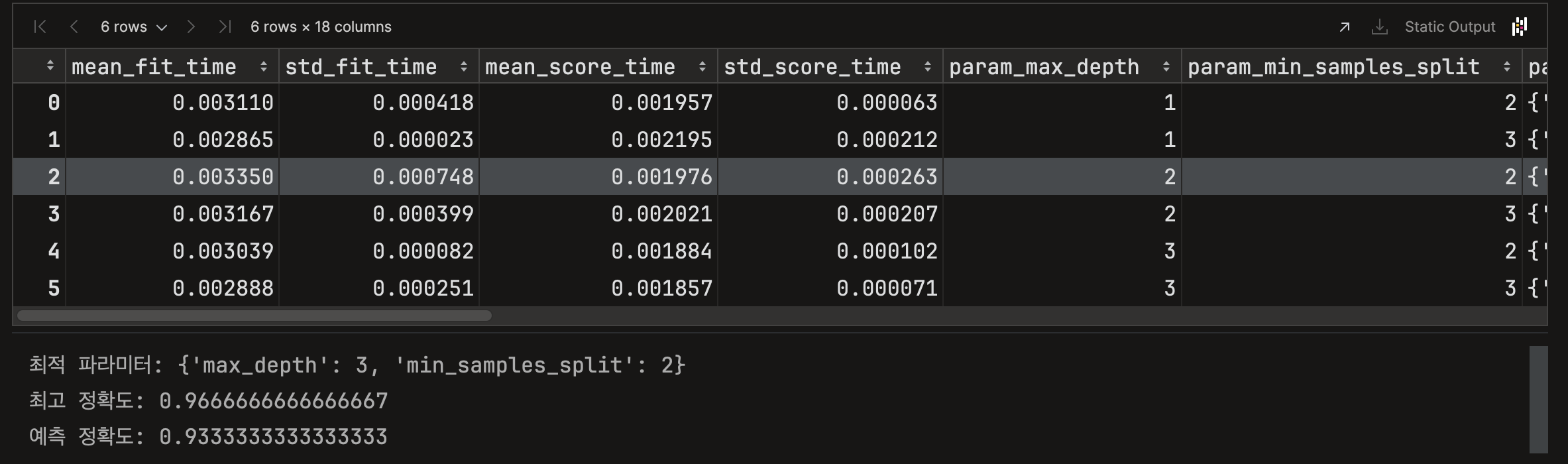
이 경우에는 최적 하이퍼 파라미터가 max_depth = 3, min_samples_split = 2인 경우에 가장 최적이라는 결과가 나왔고, 그 때의 예측 정확도는 0.97을 가진다.