[논문 리뷰] QA-GNN: Reasoning with Language Models and Knowledge Graphs for Question Answering (NAACL 2021)

KG의 subgraph를 topic entities로 찾아 few-hop 이웃 탐색
특히 entities 또는 hops 수가 늘어날 때, 의미상 관련이 없는 QA context를 찾음
QA context와 KG를 두 개로 구별해서 다룸
QA context에 LM, KG에 GNNs. 그리고 상호 업데이트 또는 결합을 하지 않음

QA-GNN : end-to-end LM + KG

QA context를 LM을 통해 encoding, 이를 따라 KG subgraph를 탐색

두 가지 핵심 insigths

Relevance scoring

주어진 QA context에 따라 중요도가 다를 수 있어서, relevance scoring을 도입한다. QA context와 entity를 합쳐 KG subgraph의 각각의 entity의 점수를 매기고, 사전 학습된 LM으로 likelihood를 계산한다. 이것이 KG 상의 weight information을 제공한다.

Joint reasoning

QA context와 KG의 joint graph representation.

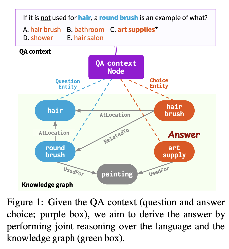
QA context를 explicit하게 추가적인 node (QA context node)로 보고, Figure 1 처럼 KG subgraph 안 의topic entities와 연결한다. (working graph) → 두 양식을 하나로 통합

Relevance score를 통해 각각의 node의 feature을 증강하고, 새로운 attention 기반의 GNN module을 사용한다. 두 source의 정보를 동시에 업데이트 함으로서 둘 사이의 간격을 좁힌다.

세 가지 datasets에서 실험

CommonsenseQA → 상식
Open-BookQA → 상식
MedQA-USMLE → 의학

LM Baseline은 물론 기존의 LM + KG model보다 훨씬 좋은 성능을 보였다.

2 Problem statement

language model의 정의

f_{\text{head}}(f_{\text{enc}}(\mathbf x))

$f_{\text{enc}}$ → encoder, textual input $\mathbf{x}$ 을 contextualized vector representation $\mathbf h^{\text{LM}}$
$f_{\text{head}}$ → 이 표현을 원하는 task에 적용시킴

이 연구에서는 $f_{\text{enc}}$ 로 masked LM (e.g.,RoBERT) 사용

$\mathbf{h}^\text{LM}$ 에서 output representation은 앞에 [CLS] token을 붙임

Knowledge graph는 multi-relational $\mathcal {G=(V,E)}$

$\mathcal V$ → KG 안의 entity nodes의 set
$\mathcal{E\subseteq V \times R \times V}$ 는 $\mathcal V$ 안의 연결된 nodes의 edges의 set ( $\mathcal R$ 은 relation type의 집합)

주어진 질문 $q$ , answer choice $a\in \mathcal C$ 와 주어진 KG $\mathcal G$ 를 연결하는 것은 이전 연구(KagNet) 방식을 사용한다.

question에서 언급된 KG entities (question entites) : $\mathcal V_q\subseteq\mathcal V$ (Figure 1에서 blue)
answer choice에서 언급된 KG entities (answer choice entities) : $\mathcal V_a\subseteq\mathcal V$ (Figure 1에서 Red)
둘 다 표현 할 때 (topic entities) : $\mathcal V_{q,a}:=\mathcal V_q \cup\mathcal V_a$

question-choice 쌍을 위해 $\mathcal G$ 에서 subgraph를 추출, $\mathcal G^{q,a}_{\text{sub}}=(\mathcal V^{q,a}_{\text{sub}},\mathcal E^{q,a}_{\text{sub}})$

이는 $\mathcal V_{q,a}$ 사이의 모든 k-hop paths로 구성된다.

3 Approach: QA-GNN

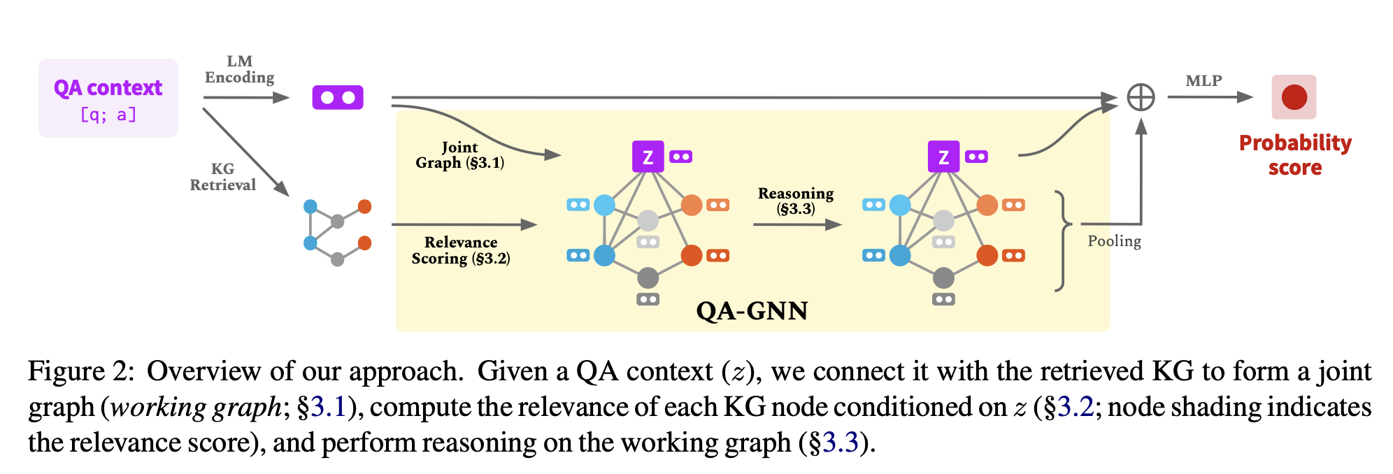
Figure 2처럼, 질문과 answer choice a가 주어졌을 때, QA context [q; a]를 얻기 위해 concatenate

주어진 QA context가 LM과 KG 양 쪽의 지식을 사용하기 위해 다음과 같은 단계를 거친다.

QA context의 representation을 얻기 위해 LM을 사용, KG에서 subgraph $\mathcal G_{\text{sub}}$ 를 탐색한다.
QA context node $z$ , 이를 topic entites $\mathcal V_{q,a}$ 에 concatenate.
이를 통해 두 source의 knowledge 사이의 joint graph를 만든다. (working graph, $\mathcal G_W$ ) → 3.1절
QA context node와 $\mathcal G_W$ 사이의 relationship을 얻기 위해 LM을 사용해 relevance score, 이 점수를 각각의 node의 추가적인 feature로 사용 → 3.2절
여러 차례 $\mathcal G_W$ 에서 message passing을 수행하는 attention-based GNN module → 3.3절
LM representation, QA context node representation, pooled working graph representation을 사용해 마지막 예측 생성 → 3.4절

computational complexity 얘기는 3.5절, 왜 우리의 models이 GNN을 사용했는지는 3.6절에서 다루어 본다.

3.1 Joint graph representation

두 source의 정보 사이의 joint reasoning space를 만들기 위해, explicit 하게 그들을 common graph structure에 연결한다.

QA context를 표현하는 새로운 QA conext node $z$ 를 만들고, 이를 KG subgraph $\mathcal G_{\text{sub}}$ 의 각각의 topic entity $\mathcal V_{q,a}$ 와 새로운 두 개의 relation type $r_{z,q}$ 와 $r_{z,a}$ 를 사용해서 연결

이는 entity가 QA context에서 question 부분인지 answer 부분인지에 따라 QA context와 KG 안의 relevant entities 사이의 relation을 표현한다.

이 연결이 QA context와 KG를 통틀어 reasoning space (working memory)를 제공하기에, working graph라는 용어로 정의한다.

$\mathcal G_W=(\mathcal V_W, \mathcal E_W)$
$\mathcal V_W=\mathcal V_{\text sub}\cup\{z\}$
$\mathcal E_W=\mathcal E_\text{sub}\cup\{(z,r_{z,q},v)|v\in \mathcal V_q\}\cup\{(z,r_{z,a},v)|v\in \mathcal V_a\}$

$\mathcal G_W$ 속의 각각의 node는 다음 4가지 중 하나에 해당한다 : $\mathcal T=\mathbf{\{Z,Q,A,O\}}$ . 각각 의미하는 바는,
context node $z$ : purple
$\mathcal V_q$ 안의 nodes : blue
$\mathcal V_a$ 안의 nodes : red
나머지 : gray

QA context node $z$ 의 text → text( $z$ )

KG node $v\in\mathcal V_{\text{sub}}$ 의 text → text( $v$ )

$z$ 의 node embedding은 QA context ( $z^{\text{LM}}=f_{\text{enc}}(\text{text}(z))$ )의 LM representation으로 초기화

각각의 $\mathcal G_{\text{sub}}$ 의 node는 그것의 entity embedding (4.2절)로 초기화

다음으로 이어지는 부분에서, working graph에 주어진 (question, answer choice) 쌍에서 score를 매길 것이다.

3.2 KG node relevance scoring

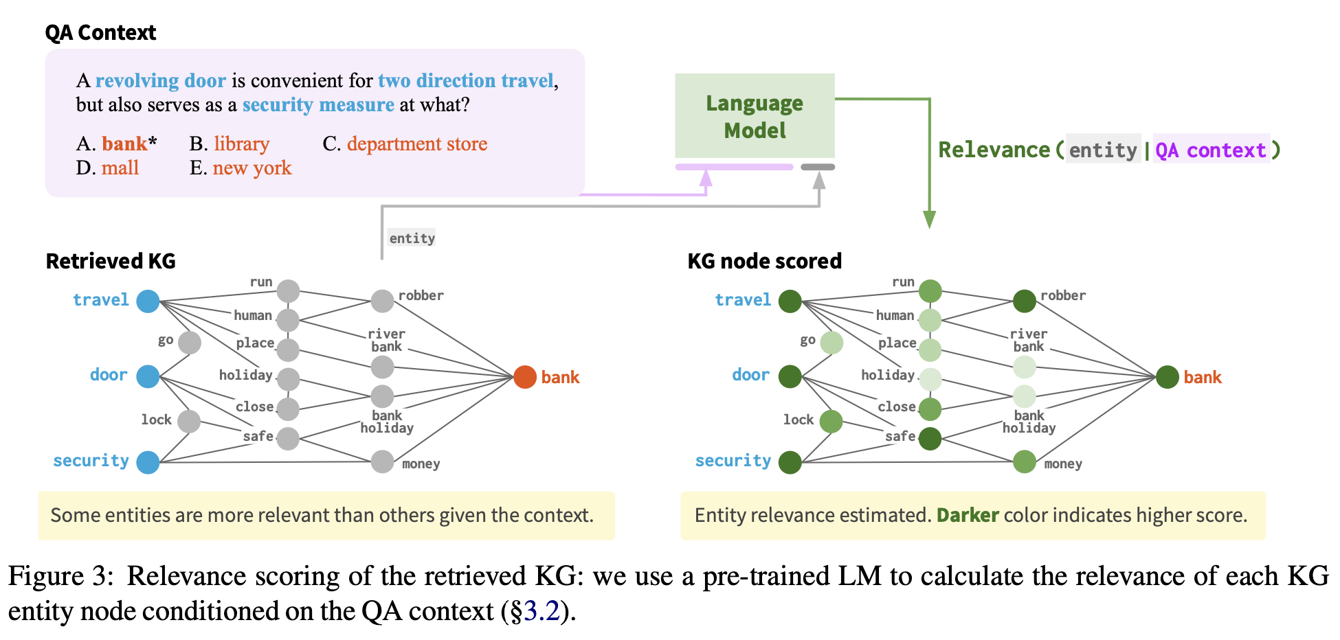
Heuristic 하게 선택된 KG subgraph $\mathcal G_{\text{sub}}$ 의 많은 노드는 현재 QA context에서 연관이 없다.

Figure 3처럼, 의미 없는 정보를 담고 있는 노드가 많다. 이러한 연관이 없는 노드들은 특히 $\mathcal V_{q,a}$ 이 클 때, overfitting 또는 불필요하게 어려운 reasoning을 하게 된다.

node relevance scoring을 제안. pre-trained language model을 사용해서, QA context에 상황에서 각각 KG node $v\in\mathcal V_{\text{sub}}$ 의 연관성을 scoring한다. 각각의 node v에 대해, entity text(v)를 QA context text(z)와 concatenate 해 relevance score를 계산한다:

\rho_v = f_{\text{head}}(f_{\text{enc}}([\text{text}(z);\text{text}(v)]))

$f_{\text{head}}\circ f_{\text{enc}}$ 은 LM에 의해 계산된 text(v)가 나올 확률

이 relevance score $\rho_v$ 는 주어진 QA context에서 각각의 KG node의 중요성을 표현하고, working graph $\mathcal G_W$ 의 reasoning 또는 pruning에 사용된다.

3.3 GNN architecture

working graph $\mathcal G_W$ 에서 reasoning을 수행하기 위해, GAT에 기반한다. 이는 graph의 이웃들 사이의 반복적인 message passing을 통해 node representations을 만든다.

특히, L-layer QA-GNN에서, 각각의 layer에서, 각각의 node $t\in\mathcal V_W$ 의 representation $h^{(l)}_t\in\mathbb R^D$ 를 다음 식으로 업데이트 한다.

\bold h^{(l+1)}_t = f_n(\sum_{s\in\mathcal N_t\cup\{t\}}\alpha_{st}\bold m_{st})+\bold h^{(l)}_t

$\mathcal N_t$ 은 node t의 이웃 node
$m_{st}\in\mathbb R^D$ 는 각각의 이웃 node s에서 t까지 전달된 message
$\alpha_{st}$ 는 s에서 t로 오는 각각의 message $m_{st}$ 를 scale 하는 attention weight

message의 합은 2-layer MLP, $f_n:\mathbb R^D\rightarrow\mathbb R^D$ 를 batch normalization과 함께 통과한다.

각각의 node $t\in\mathcal V_W$ 에 대해, $h^{(0)}_t$ 를 그것의 초기 node embedding (3.1절)을 $\mathbb R^D$ 로 map하는 linear transformation $f_h$ 을 사용해 설정한다.

결정적으로, GNN message passing이 working graph에서 일어나기 때문에, QA context와 KG의 representation을 결합적으로 사용하고 update한다.

expressive message ( $m_{st})$ 와 attention ( $\alpha_{st}$ )는 밑에서 계산한다.

Node type & relation-aware message.

$\mathcal G_W$ 가 multi-relational graph이기 때문에, source node에서 targe node로 전달되는 message는 edge와 source/target node의 relation type을 확인해야 한다.

이를 위해, 먼저 node s에서 node t의 relation embedding $r_{st}$ 뿐만 아니라, 각각의 node t의 type embedding $u_t$ 도 얻는다.

\mathbf{u}_t=f_u(\mathsf u_t),\quad \textit{\textbf{r}}_{st}=f_r(\text e_{st}, \text u_s, \text u_t)

$\text u_s, \text u_t \in \{ 0,1\}^{|\mathcal T|}$ → s와 t의 node type을 가리키는 one-hot vectors
$\text{e}_{st}\in \{0,1\}^{|\mathcal R|}$ → edge (s, t)의 relation type을 가리키는 one-hot vectors
$f_u:\mathbb R^{|\mathcal T|}\rightarrow\mathbb R^{D/2}$ → linear transformation
$f_r:\mathbb R^{|\mathcal R|+2|\mathcal T|}\rightarrow\mathbb R^{D}$ → 2-layer MLP

이후 우리는 s에서 t로 오는 message를 계산한다.

\textit{\textbf{m}}_{st}=f_m(\textit{\textbf{h}}^{(l)}_s, \textit{\textbf{u}}_s, \textit{\textbf{r}}_{st})

$f_m:\mathbb R^{2.5D}\rightarrow\mathbb R^{D}$ → linear transformation

Node type, relation, and score-aware attention.

Attention은 이상적으로 그들의 node types, relations, node relevance score로 정보가 주어지는 두 노드 사이의 연결의 강도를 알아낸다.

먼저 각 node t의 relevance score를 embed한다.

\boldsymbol\rho_t =f_{\rho}(\rho_{t})

$f_{\rho}:\mathbb R\rightarrow\mathbb R^{D/2}$ → MLP

node s에서 node t로의 attention weight $\alpha_{st}$ 를 계산하기 위해, query와 key vectors $\textit{\textbf{q}},\textit{\textbf{k}}$ 를 얻는다.

\textit{\textbf{q}}_s=f_q(\textit{\textbf{h}}^{(l)}_s, \textit{\textbf{u}}_s,\boldsymbol\rho_s),\\ \textit{\textbf{k}}_t=f_k(\textit{\textbf{h}}^{(l)}_t, \textit{\textbf{u}}_t,\boldsymbol\rho_t,\textit{\textbf{r}}_{st})

$f_q:\mathbb R^{2D}\rightarrow \mathbb R^{D}$ , $f_k:\mathbb R^{3D}\rightarrow\mathbb R^D$ 는 linear transformation

Attention weight는 다음과 같다.

\alpha_{st}=\frac{\exp(\gamma_{st})}{\sum_{t^{\prime}\in \mathcal N\cup\{s\}}\exp(\gamma_{st^{\prime}})},\quad\gamma_{st}=\frac{q_s^{\top}k_t}{\sqrt D}.

3.4 Inference & Learning

question q와 answer choice a가 주어졌을 때, 정답인 $p(a|q)\propto\exp(\text{MLP}(\textit{\textbf{z}}^{\text{LM}},\textit{\textbf{z}}^{\text{GNN}},\textit{\textbf{g}}))$ 가 될 확률을 QA context와 KG의 정보를 둘 다 사용해 계산한다.

$\textit{\textbf{z}}^{\text{GNN}}=\textit{\textbf{h}}^{(L)}_z$
$\textit{\textbf{g}}$ → $\{\textit{\textbf{h}}^{(L)}_v|v\in\mathcal V_{\text{sub}}\}$ 의 pooing

Training data에서, 각각의 question은 answer choices의 set을 가지고 있고, 하나의 올바른 정답을 가진다.

LM, GNN componets end-to-end 둘 다 cross entropy loss로 최적화 한다.

3.5 Computation complexity

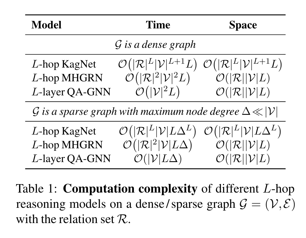
Table 1에서 이전 연구 KagNet, MHGRN과 time / space 복잡도를 비교했다.

우리 연구는 다른 relation type을 RGCN 또는 MHGRN 처럼 각각의 relation에 독립된 graph networks를 디자인 하지 않고, 다른 edge embedding을 통해 다루기 때문에, relation의 수에 constant하고, nodes의 수에 linear 하다. MHGRN과 같은 공간 복잡도를 달성했다.

3.6 Why GNN for question answering?

최근 연구는 GNNs이 다양한 graph algorithm을 modeling하는데 효과적임을 보였다.

예시 : knowledge graph reasoning (KG 상에 logical queries 실행 같은)

V_{?}.\exist V:\text{Located(Europe, \it V)}\wedge\neg\text{Held(World Cup, \it V)}\wedge\text{President}(V, V_?)

\textit{("Who are the presents of European countries that have \textbf {not} held the World Cup?")}

이러한 logical queries를 input “question”으로 봐서, QA-GNN을 KG 상의 logical queries 실행 task를 학습 하는데 pilot study를 수행했다 - entities의 부정 또는 multi-hop relations을 포함하는 복잡한 queries를 가지고 있다.

QA-GNN가 LM 뿐만 아니라 GNN 보다 성능이 좋았다.

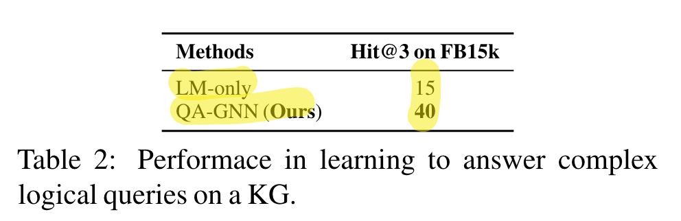
GNNs이 complex query answering을 modeling하는데 정말 유용함을 확인시켜준다.

QA-GNN이 complex natural language question answering에도 유용할 것이라는 insight를 준다, 이는 logical (KG) 대신 soft queries (natural language)를 실행하는 것이라 볼 수 있다.

“KG query excution” 직관에 따라, KG와 GNN이 model이 question 내의 언급된 entities에 대한 reson을 위한 발판을 제공할 수 있다는 설명을 또한 그릴 수 있다. 4.6.3절에서 더욱 분석한다.

4 Experiments

4.1 Datasets

QA-GNN을 세 가지 answering datasets에서 비교

CommonsenseQA
OpenBookQA
MedQA-USMLE

CommonsenseQA는 5지선다 객관식 QA task. 상식으로부터 추론이 필요. 12,102개의 질문.

test set은 공개 되지 않음, model prediction은 2주에 1번 공식 leaderboard에 집계됨.

핵심 실험을 in-house(IH) data splits 상에서 수행했고, 최종 시스템을 공식 test set에도 올림.

OpenBookQA는 4지선다 객관식 QA task. 기초 과학 지식으로부터 추론 필요. 5,957개의 질문.

official data를 사용

MedQA-USMLE는 4지선다 객관식 QA task. biomedical과 clinical 지식을 필요.

미국 의학 면허 시험에서 왔음. 12,723개의 질문. original data를 사용.

4.2 Knowledge graphs

CommonsenseQA, OpenBookQA → ConcepNet (일반 영역 지식 그래프)을 structured knowledge source $\mathcal G$ 로 사용. 799,273 nodes, 2,487,810 edges. Node embedding은 pre-trained LMs을 ConceptNet의 모든 triples에 적용하고 각각 entity의 pooled representation을 얻는 “**Scalable Multi-Hop Relational Reasoning for Knowledge-Aware Question Answering**” (Feng, EMNLP 2020)의 연구에서 준비된 entity embedding으로 초기화.

MedQA-USMLE → Disease Database에서 자체 제작한 knowledge graph. 9,958 nodes, 44,561 edges. Node embedding은 SapBERT라는 이름의 entity의 pooled representation으로 초기화 됨.

주어진 QA context에서, subgraph $\mathcal G_{\text{sub}}$ 를 Feng의 연구에서 묘사된 pre-processing 단계를 따라 찾는다. (hop size $k=2$ ). 그 후 3.2절에서 계산된 relevance score에 따라 상위 200 nodes가 남도록 $\mathcal G_{\text{sub}}$ 를 prune. 앞으로 4절에서 “KG”는 $\mathcal G_{\text{sub}}$ 를 의미한다.

4.3 Implementation & training details

dimension : $D=200$
layer의 수 : $L=5$
각각의 layer의 dropout rate : $0.2$
RAdam 사용
두 개의 GPUs (GeForce RTX 2080 TI)
~20시간 소요
batch size : $\{32,64,128,256\}$
LM module의 learning rate : $\{5e-6,1e-5,2e-5,3e-5,5e-5\}$
GNN module의 learning rate : $\{2e-4,5e-4,1e-3,2e-3\}$

이 hyperparemeters는 development set 상에서 tuned됨

4.4 Baselines

Fine-tuned LM.

KGs의 역할을 연구하기 위해, KG를 사용하지 않는 vanilla fine-tuned LM과 비교.

CommonsenseQA → RoBERTa-large
OpenBookQA → RoBERTa-large 와 AristoRoBERTa
MedQA-USMLE → SOTA biomedical LM인 SapBERT

Existing LM+KG models.

high-level framework는 공유하지만 QA-GNN에서 KG 상의 reason이 (Figure 2의 노란 부분) 다른 LM+KG models과도 비교.

Relation Network (RN)
RGCN
GconAttn
KagNet
MHGRN

1, 2,3은 relation-aware GNNs을 위한 KGs

4, 5는 KG에서 further model paths.

MHGRN은 LM+KG framework에서 현재 최고 성능.

공평한 비교를 위해, baseline과 우리 모델 모두 같은 LM을 사용.

QA-GNN과 이것들이 가장 중요한 차이는 relevance scoring을 수행하지 않고, QA context에서 joint updates를 하지 않는다는 점 (3절)

4.5 Main results

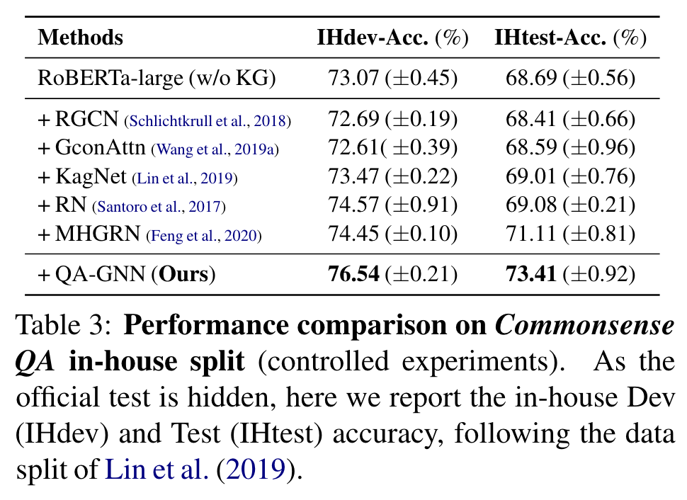
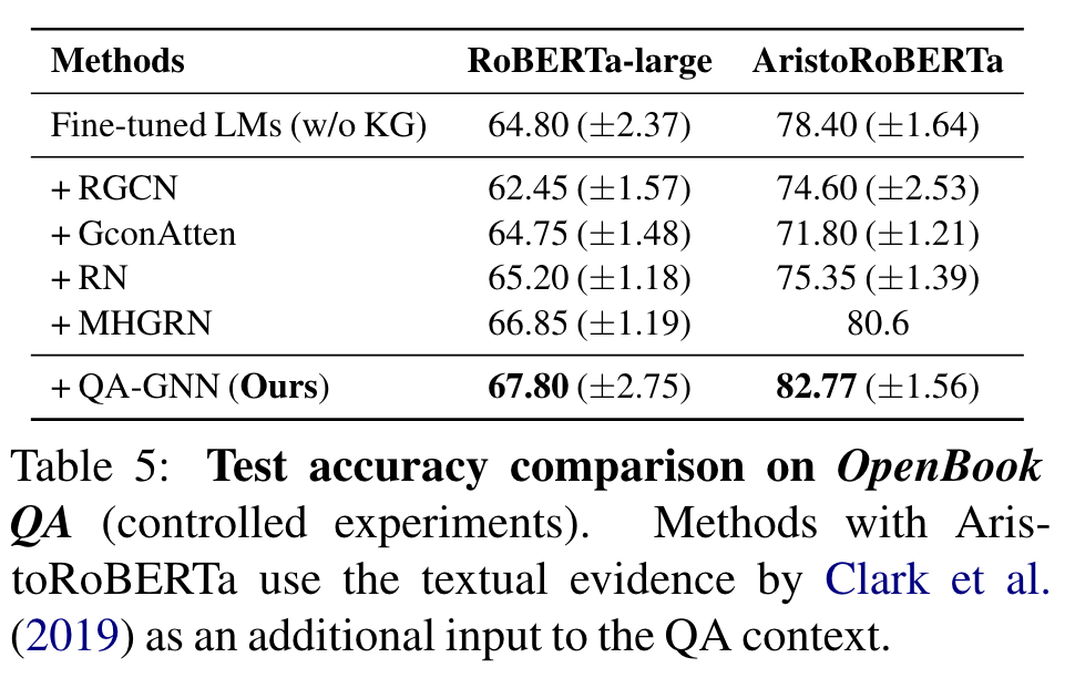
Table 3, 5는 각각 CommonsendQA, OpenBookQA의 결과.

양 datasets에서, fine-tuned LM과 현존 LM+KG models과 비교해서 일관된 향상

CommonsenseQA

RoBERTa +4.7%
MHGRN (현존 최고 LM+KG) + 2.3%

MHGRN에서 성능 향상은 QA-GNN이 현존 최고임을 보인다.

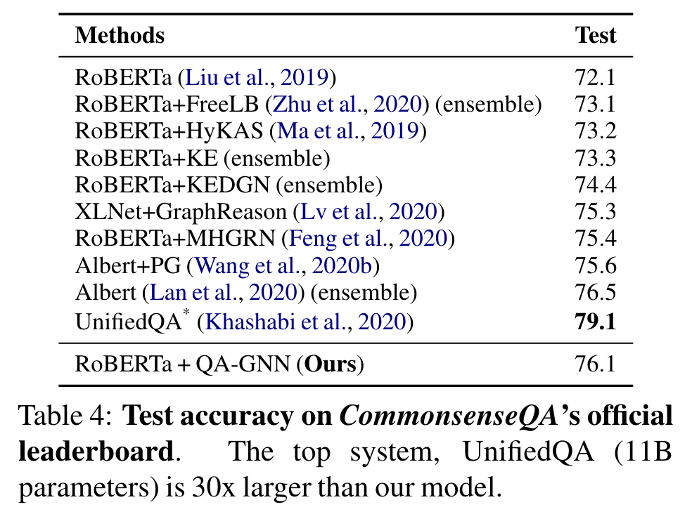
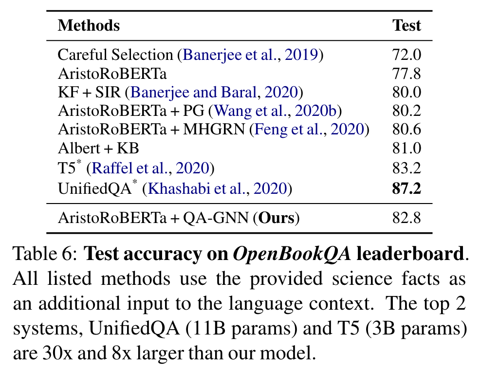
다른 official leaderboards에서도 좋은 성과를 또한 달성

최고 두 system, T5, UnifiedQA는 더 많은 데이터에서, 8배에서 30배 많은 parameters를 사용. (우리는 ~360M parameters)

이것들과 ensemble systems을 제외하면, 우리의 모델은 규모와 데이터 양에서 비교할 법 하고, 두 데이터 set에서 최고 성능을 보인다.

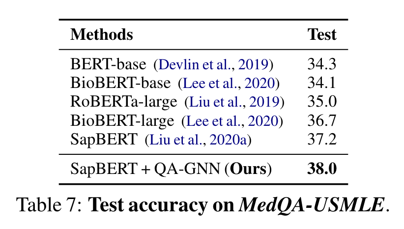
Table 7은 MedQA-USMLE의 결과. SOTA LMs (SapBERT)보다 좋은 성과. 이 결과는 우리의 방식이 다른 domains에서 효과적인 LMs과 KGs의 augmentation임을 제시한다.

4.6 Analysis

4.6.1 Ablation studies

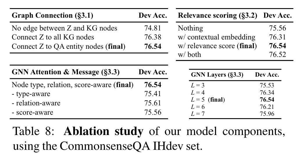
Table 8은 각각 model 요소들에서 수행된 ablation study의 요약. CommonsenseQA IHdev set 사용.

Graph connection (왼쪽 위 표): QA-GNN의 첫번째 핵심 요소는 QA context인 $z$ node와 KG 상의 QA entity nodes $\mathcal V_{q,a}$ 를 concat (3.1절). 이 edges가 없다면, QA context와 KG는 그들의 representations을 상호 update 할 수 없고, 성능이 하락 한다: $76.5\%\rightarrow74.8\%$ , 이는 기존 LM+KG system, MHGRN과 유사. 만약 $z$ 를 오직 QA entities가 아니라 전체 KG의 nodes와 연결한다면, performance가 조금 하락 ( $-0.16\%$ )

KG node relevance scroing (오른쪽 위 표): KG nodes와의 relevacne scoring (3.2절)이 성능 향상을 보이는 것을 발견: $75.56\%\rightarrow76.54\%$ . Eq. 1의 relevance scoring이 다양하기 때문에, 각각의 node $v\in\mathcal V_{\text{sub}}$ 의 contextual embedding $\textit{\textbf{w}}_v$ 를 구하고 node features을 더하는 실험도 진행해 봤다:

GNN architecture (하단 표): GNN에서 attention과 message computation에서 온 node type, relation, relevance score (3.3절)을 ablate했다. 모든 이런 feauters가 성능 향상을 했음을 제안한다. GNN Lyaers에 대해서는, dev set에서 $L=5$ 가 가장 잘 작동함을 확안했다. 우리의 직관으로는 5 layers가 QA context(z)와 KG 사이의 다양한 message passing 또는 reasoning patterns을 가능하게 했다고 본다, “z → 3 hops on KG nodes → z” 같이.

4.6.2 Model interpretability

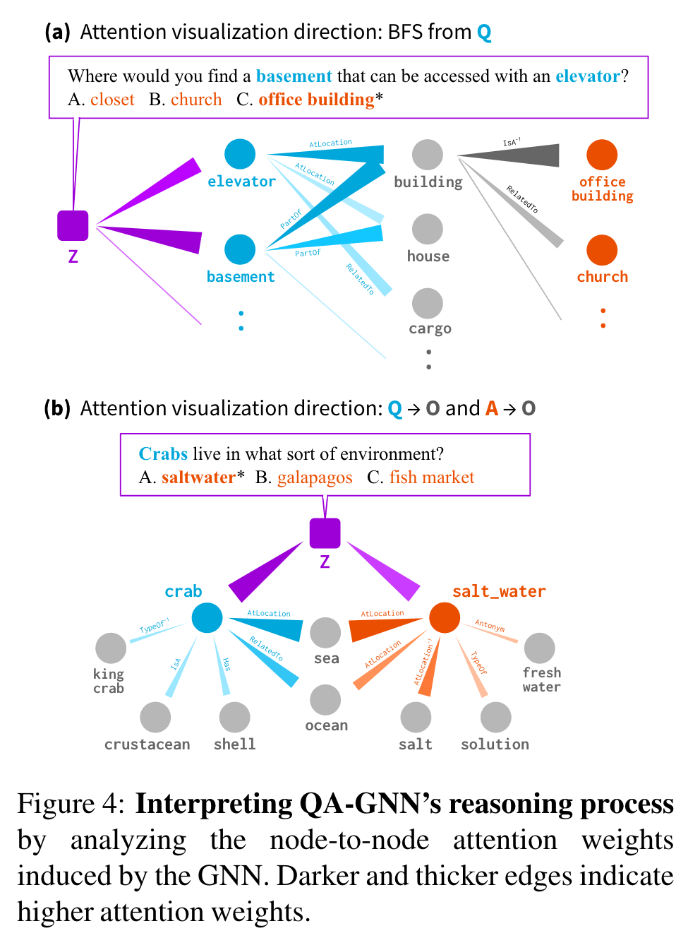
QA-GNN의 reasoning process를 GNN에서 유도된 node-to-node attention weights를 분석해서 해석하는 것이 목표.

Figure 4는 두 예시를 보임.

(a), Best First Search (BFS)를 working graph에서 수행. QA context node (Z; 보라)에서 Question entity node (Q; 파랑) 에서 Other (O; 회색) 또는 Answer Choice (A; 오렌지)까지의 높은 attention weight를 추적. 이는 QA context z는 KG 상의 “elevator”와 “basement”를 방문, “elevator” 와 “basment”는 둘 다 “building”을 강하게 방문, “building”은 “office building”을 방문, 이는 최종 정답이 된다.

(b), BFS를 두 방향에서 attention weights를 추적하는데 사용: Z→Q→O와 Z→A→O. 이는 KG 상의 concept(”sea”와 “ocean”)이 QA context에서 필수적으로 언급되지 않았지만, question entity (”crab”)와 answer choice entity(”salt water”)사이의 연결 다리가 되어 주었다.

기존 연구와 달리 QA-GNN은 경로에 특징적이지 않고, 더 일반적인 reasoning structures를 찾는다. (a의 예시처럼 KG subgraph가 다중 anchor nodes가 있을 때)

4.6.3 Structured reasoning

Structure reasoning (negation 또는 entity substituion을 정확히 다루는 것)은 robust predictions에 중요하다. QA-GNN의 structured reasoning 능력을 분석하고 baselines과 비교한다. (fine-tuned LMs과 현존 LM+KG models)

Quantitative analysis.

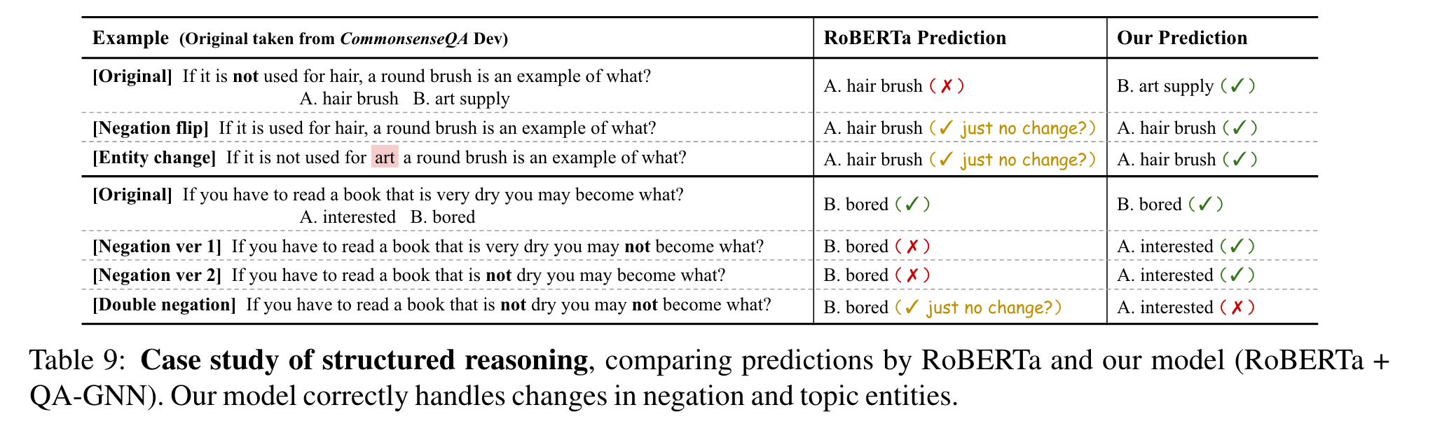
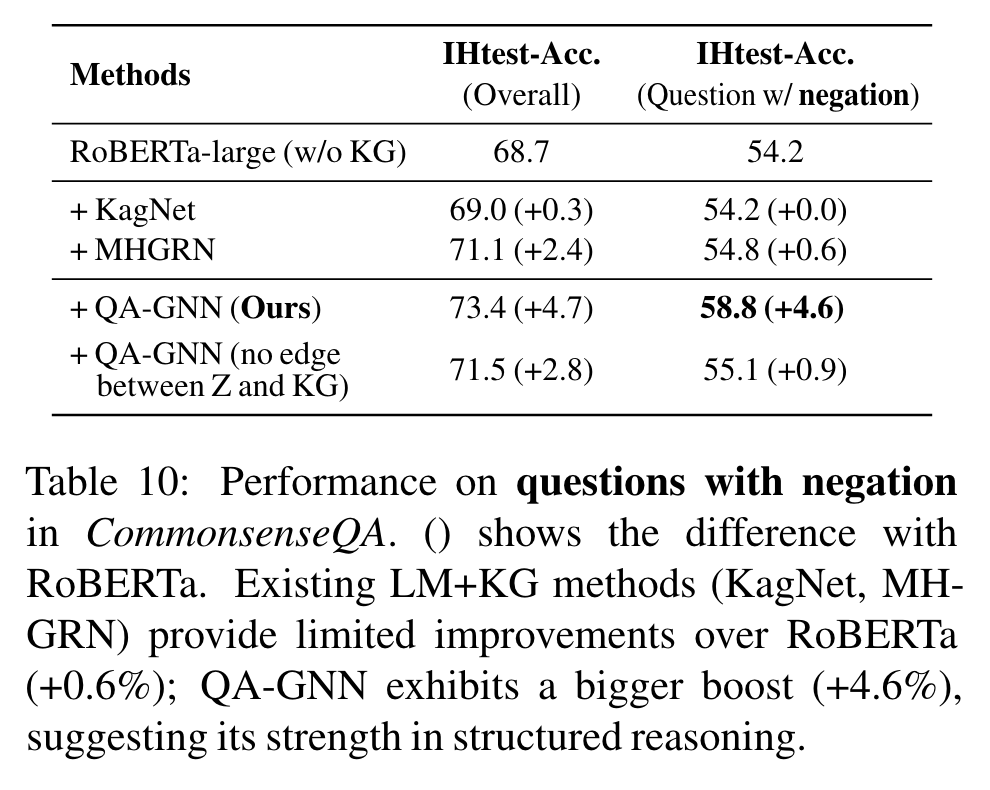
Table 10은 negation words를 포함한 질문에서의 performance 비교 - CommonsenseQA IHtest set에서 발췌. 기존 LM+KG models은 negation 질문에서 RoBERT와 비교할 시 제한된 향상만을 보임 (+0.6%). 반면, QA-GNN은 더 큰 향상 (+4.6%), 이는 structured reasoning에 더 강함을 보임.

QA-GNN의 joint updates가 model이 언어 상의 문맥적 뉘앙스를 통합하게 했다고 가정한다. 이 가설을 더 연구하기 위해, z와 KG nodes 사이의 연결을 끊어 봄 (Table 10): 이전 연구 MHGRN과 negation performance가 유사해 짐, 이는 joint message passing이 structured reasoning에 도움이 된다는 것을 제안함.

Qualitative analysis.

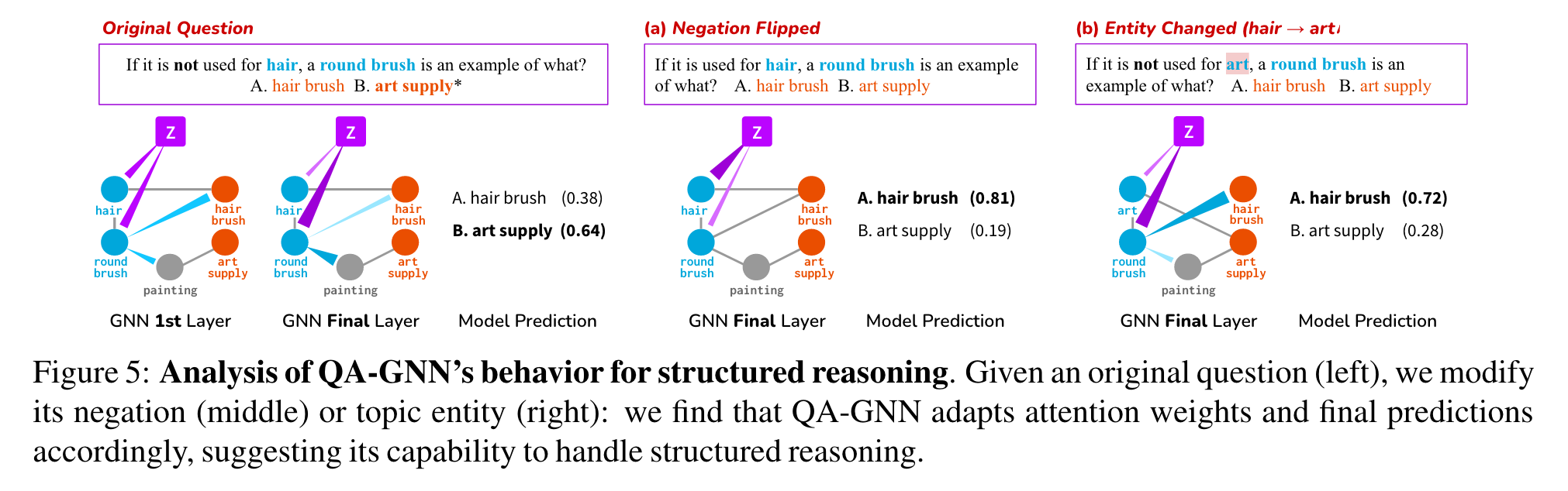
Figure 5는 structured reasoning을 위한 우리 model의 행동을 분석한 case study. 왼쪽의 질문은 negation “not used for hair”, 정답은 “B. art supply”. QA-GNN의 첫번째 Layer에서, z에서 question entities (”hair”, “round brush”)의 attentin이 퍼지는 것을 관찰. 여러 단계가 지난 후, z는 “round brush”에 GNN의 마지막 단계에서 강하게 attentd하지만, negated entity “hair”에는 약하게 attend. 모델은 정확하게 답을 맞췄다.

다음으로, 원래 질문이 있을 때, (a) negation을 누락하거나 (b) topic entity (”hair” → “art”)로 바꿨다.

(a)에서, z는 이제 negated 되지 않는 hair을 강하게 attend. 올바른 정답 “A. hair brush” 맞춤.

(b)에서, QA-GNN이 기존 질문과 같은 구조를 인식하는 것을 관찰함: z는 이전처럼 negated entity (”art”)는 약하게 참고하고, 모델은 정확한 예측을 한다.

Table 9는 추가적인 예시를 보이는데, QA-GNN의 예측을 LM baseline과 비교한다. RoBERTa는 기존 질문에 수정을 가하는 것과 상관 없이 같은 예측을 만드는 것을 관찰; 반면, QA-GNN은 수정에 맞춰 올바른 정답을 찾느다. (맨 밑의 double negation은 그렇지 않다. 미래의 연구 과제)

4.6.4 Effect of KG node relevance scoring

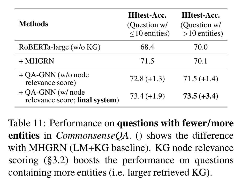
KG node relevance scoring (3.2절)이 탐색된 KG ( $\mathcal G_{\text{sub}}$ )가 클 때 유용하다는 것을 확인했다.

Table 11은 더 적고 (≤ 10) 또는 많은 (>10) entities가 CommonsenseQA IHtest set에 있을 때, model performance를 보여준다. (앞 뒤 90, 160 nodes). MHGRN 같은 현존 LM+KG models은 탐색된 KG의 size와 noisiness 때문에 더 많은 entities가 있을 경우 제한된 performance를 달성한다: 70.1% 정확도 vs 적은 entities에서 71.5% 정확도. KG node relevacne scoring는 이 bottle을 완화시키고, accuracy 격차를 줄인다: more/fewer에서 각각 73.%와 73.4%.

Knowledge-aware methods for NLP.

NLP를 Knowledge로 augement하는 연구가 존재. LM’s의 잠재력을 최신 knowledge base로 사용. 더 명시적이고 해석 가능한 지식을 제공하기 위해, structure knowledge graph를 LM에 통합하고자 하는 노력.

Question answering with LM+KG.

기존 연구가 있었음. 우리의 고유한 능력

QA context와 KG의 joint graph, 상호 representation update
language-conditioned KG node relevance scoring

scoring 또는 pruning KG nodes/paths는 QA context가 아닌 graph-based metrics만 있었다.

Other QA tasks.

기존 연구와 달리 question answering을 LM과 KG에서 온 지식으로 해결했다.

Knowledge representations.

external textual knowledge와 structured knowledg의 joint representation에 대한 연구.

우리의 joint graph representation과 주요한 구분은 textual하고 structural knowledge가 아니라 상기 연구의 보완적인 문제에 접근하는 question과 KG를 연결하는 graph를 만들었다는 점.

Graph neural networks (GNNs).

GATs 기반의 attention-based message passing을 사용했다.

6 Conclusion

QA-GNN, LMs과 KGs를 사용하는 end-to-end question answering models. 우리의 주요 발명

Relevance scoring, KG nodes 사이의 relevance를 주어진 QA context에서 계산
Joint reasoning, working graph를 통해 두 정보의 소스 QA context와 KGs 사이의 연결, jointly하게 그들의 정보를 GNN message passing으로 update

quantitative 와 qualitative 분석 양 쪽에서, 현존하는 LM과 LM+KG models에서 question answering tasks 상에서 QA-GNN의 발전이 있음을 보였고, interpretable 하고 structured reasoning의 능력도 가지고 있음을 보였다.

References

Scalable Multi-Hop Relational Reasoning for Knowledge-Aware Question Answering

KagNet: Knowledge-Aware Graph Networks for Commonsense Reasoning

지동환

고려대학교 컴퓨터학과 19. 현재 학부 인턴. 인공지능을 공부하는 중. 주 관심사는 Graph, Vision, 그리고 TRUE AGI.

[논문 리뷰] QA-GNN: Reasoning with Language Models and Knowledge Graphs for Question Answering (NAACL 2021)

Paper-review

Abstract

1 Introduction

2 Problem statement