데이터 불러오기
https://statiz.sporki.com/
스탯티즈 사이트에서 선수 정보들을 들고와서 불러와줍니다~
import pandas as pd

picher_file_path = './picher_stats_2017.csv'
picher = pd.read_csv(picher_file_path)
데이터를 한 번 확인해보겠습니다~
print(picher.head())
print(picher.columns)
print(picher['연봉(2018)'].describe())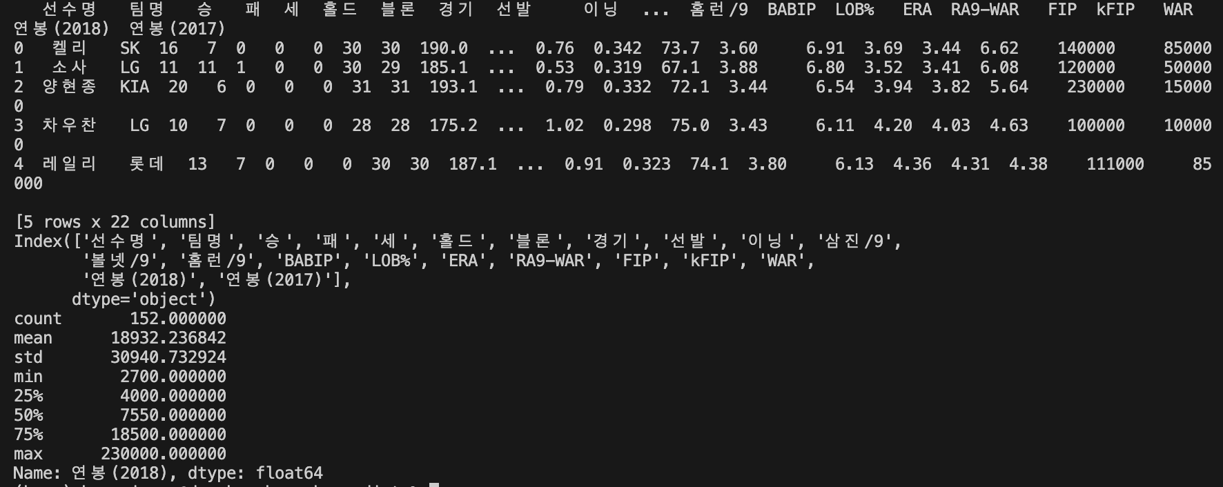
폰트 적용
그래프로 확인해보기 전에 한글 폰트를 적용 시켜보도록 하겠습니다~
import matplotlib.pyplot as plt
import matplotlib.font_manager as fm

font_path = './NanumGothic.otf'
# 폰트를 matplotlib에 등록합니다.
fm.fontManager.addfont(font_path)
plt.rc('font', family='NanumGothicOTF')
그래프 확인
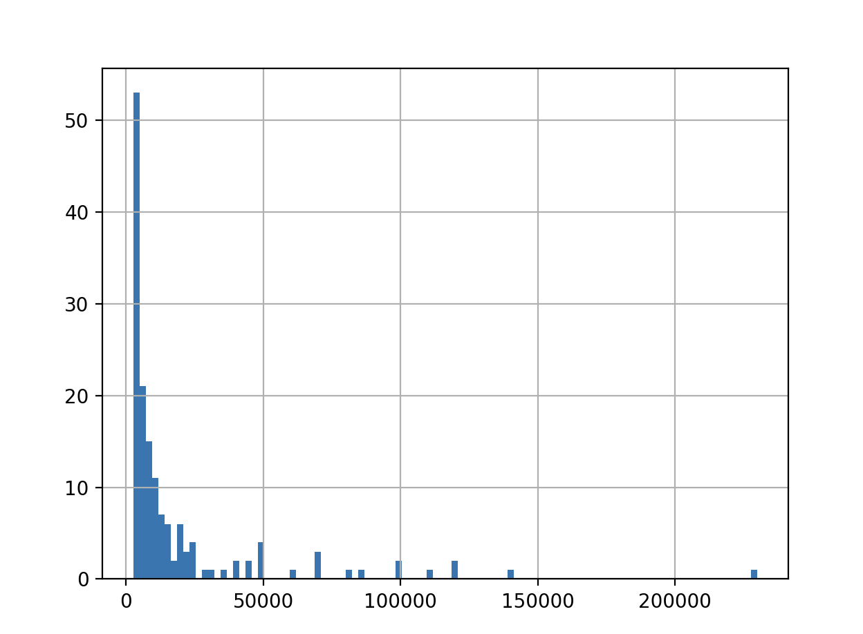
picher['연봉(2018)'].hist(bins=100)
plt.show()
picher.boxplot(column=['연봉(2018)'])
plt.show()
연봉 분포에 대한 그래프
연봉의 BoxPlot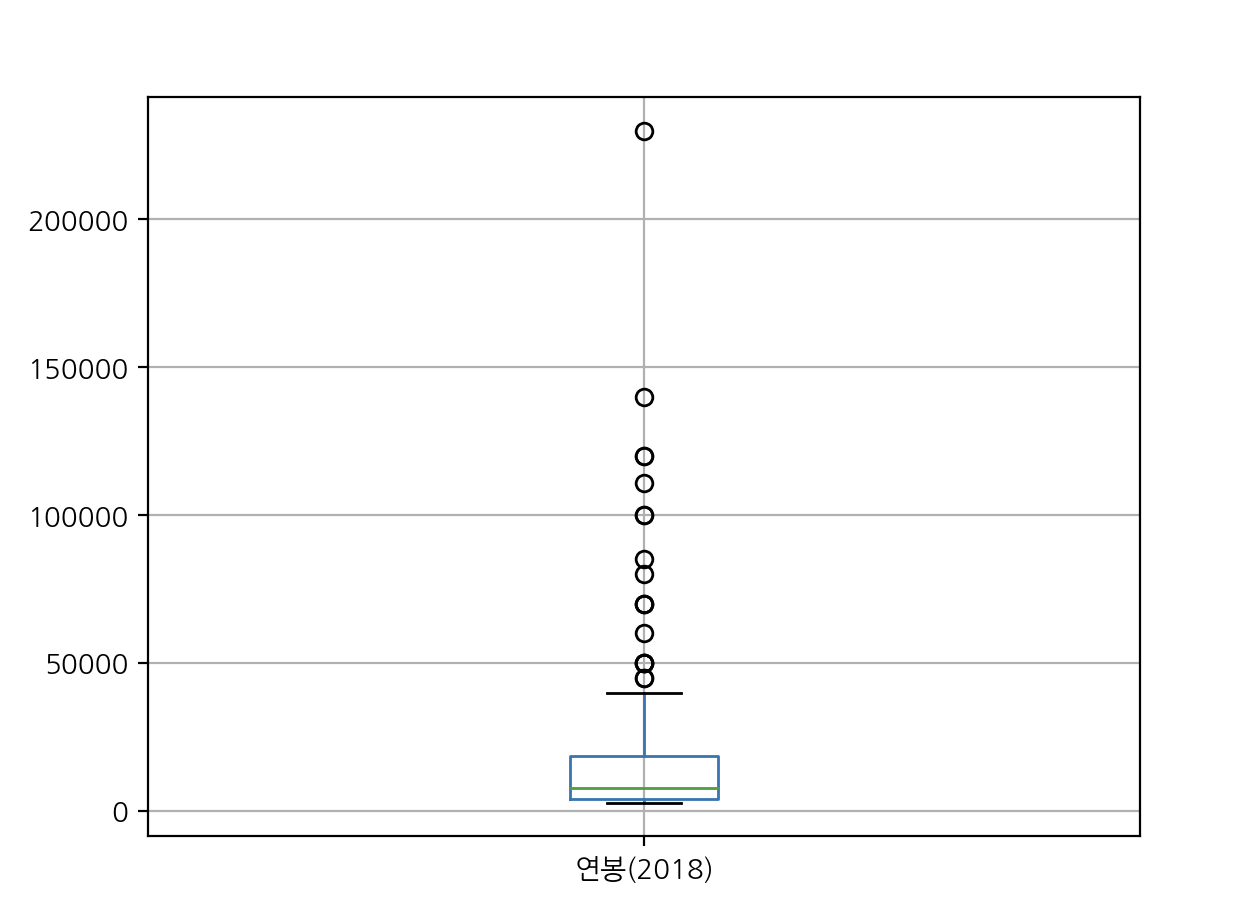
회귀분석에 사용할 피처
picher_features_df = picher[['승', '패', '세', '홀드', '블론', '경기', '선발', '이닝', '삼진/9',
       '볼넷/9', '홈런/9', 'BABIP', 'LOB%', 'ERA', 'RA9-WAR', 'FIP', 'kFIP', 'WAR',
       '연봉(2018)', '연봉(2017)']]
회귀분석에 사용할 피처들을 정리해줍니다
def plot_hist_each_column(df):
    plt.rcParams['figure.figsize'] = [20, 16]
    fig = plt.figure(1)

    # df의 column 갯수 만큼의 subplot을 출력합니다.
    for i in range(len(df.columns)):
        ax = fig.add_subplot(5, 5, i+1)
        plt.hist(df[df.columns[i]], bins=50)
        ax.set_title(df.columns[i])
    plt.show()

plot_hist_each_column(picher_features_df)
피처 각각에 대한 히스토그램을 확인해보겠습니다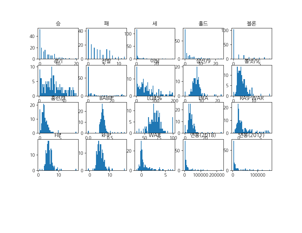
연봉 예측
본격적인 연봉예측 시간~~~
먼저 피처들을 스케일링부터 해줍니다
# pandas 형태로 정의된 데이터를 출력할 때, scientific-notation이 아닌 float 모양으로 출력되게 해줍니다.
pd.options.mode.chained_assignment = None

# 피처 각각에 대한 scaling을 수행하는 함수를 정의합니다.
def standard_scaling(df, scale_columns):
    for col in scale_columns:
        series_mean = df[col].mean()
        series_std = df[col].std()
        df[col] = df[col].apply(lambda x: (x-series_mean)/series_std)
    return df

# 피처 각각에 대한 scaling을 수행합니다.
scale_columns = ['승', '패', '세', '홀드', '블론', '경기', '선발', '이닝', '삼진/9',
       '볼넷/9', '홈런/9', 'BABIP', 'LOB%', 'ERA', 'RA9-WAR', 'FIP', 'kFIP', 'WAR', '연봉(2017)']
picher_df = standard_scaling(picher, scale_columns)

picher_df = picher_df.rename(columns={'연봉(2018)': 'y'})
picher_df.head(5)
one-hot-encoding을 통해 피처들의 단위를 맞춰서 원활한 회귀분석을 할 수 있도록 해보겠습니다
team_encoding = pd.get_dummies(picher_df['팀명'])
picher_df = picher_df.drop('팀명', axis=1)
picher_df = picher_df.join(team_encoding)

team_encoding.head(5)

picher_df.head()
회귀분석을 위해 학습 데이터와 테스트 데이터를 분리
X = picher_df[picher_df.columns.difference(['선수명', 'y'])]
y = picher_df['y']
X_train, X_test, y_train, y_test = train_test_split(X, y, test_size=0.2, random_state=19)
회귀 모델 학습
lr = linear_model.LinearRegression()
model = lr.fit(X_train, y_train)

print(lr.coef_)

print(picher_df.columns)
모델 정확성 평가
y_pred = lr.predict(X_test)

mse = mean_squared_error(y_test, y_pred)
rmse = sqrt(mse)

print(f'평균 제곱 오차(MSE): {mse}')
print(f'루트 평균 제곱 오차(RMSE): {rmse}')

test_result_df = pd.DataFrame({'실제연봉(2018)': y_test, '예측연봉(2018)': y_pred})
test_result_df = test_result_df.sort_values(by='실제연봉(2018)', ascending=False).reset_index(drop=True)
print(test_result_df.head(10))

plt.figure(figsize=(10, 6))
plt.plot(y_test.values, label='실제연봉(2018)', color='blue', alpha=0.7)
plt.plot(y_pred, label='예측연봉(2018)', color='orange', alpha=0.5)
plt.xlabel('선수 인덱스')
plt.ylabel('연봉')
plt.title('테스트 데이터에 대한 실제 연봉과 예측 연봉')
plt.legend()
plt.show()
연봉 예측
X= picher_df[lr.feature_names_in_]
predict_2018_salary = lr.predict(X)
picher_df['예측연봉(2018)'] = pd.Series(predict_2018_salary)
.
picher = pd.read_csv(picher_file_path)
picher = picher[['선수명', '연봉(2017)']]
예측 모델 평가
2018년도의 연봉 정보를 가지고 예측한 2018년도의 연봉 정보와 비교를 통해 예측 모델을 평가해볼겁니다~~
batter = pd.read_csv(batter_file_path)먼저 파일을 불러오고
X= picher_df[lr.feature_names_in_]
predict_2018_salary = lr.predict(X)
picher_df['예측연봉(2018)'] = pd.Series(predict_2018_salary)

picher = pd.read_csv(picher_file_path)
picher = picher[['선수명', '연봉(2017)']]

result_df = picher_df.sort_values(by=['y'], ascending=False)
result_df.drop(['연봉(2017)'], axis=1, inplace=True, errors='ignore')
result_df = result_df.merge(picher, on=['선수명'], how='left')
result_df = result_df[['선수명', 'y', '예측연봉(2018)', '연봉(2017)']]
result_df.columns = ['선수명', '실제연봉(2018)', '예측연봉(2018)', '작년연봉(2017)']
2018년 연봉을 예측한 데이터를 들고와서 데이터프레임이랑 합칩니다
result_df = result_df[result_df['작년연봉(2017)'] != result_df['실제연봉(2018)']]
result_df = result_df.reset_index()
result_df = result_df.iloc[:10, :]
print(result_df.head(10))

plt.show()
재계약한 선수들만 대상으로 연봉에 대한 예상과 실제 연봉입니다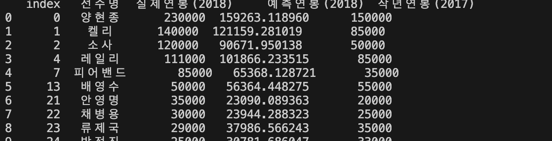
그래프로 나타내기~~~
plt.figure(figsize=(10, 6))
plt.bar(result_df['선수명'], result_df['실제연봉(2018)'], color='blue', alpha=0.7, label='실제연봉(2018)')
plt.bar(result_df['선수명'], result_df['예측연봉(2018)'], color='orange', alpha=0.5, label='예측연봉(2018)')

# 그래프 레이블과 제목 설정
plt.xlabel('선수명')
plt.ylabel('연봉')
plt.title('선수별 실제 연봉(2018)과 예측 연봉(2018)')
plt.legend()

plt.show()
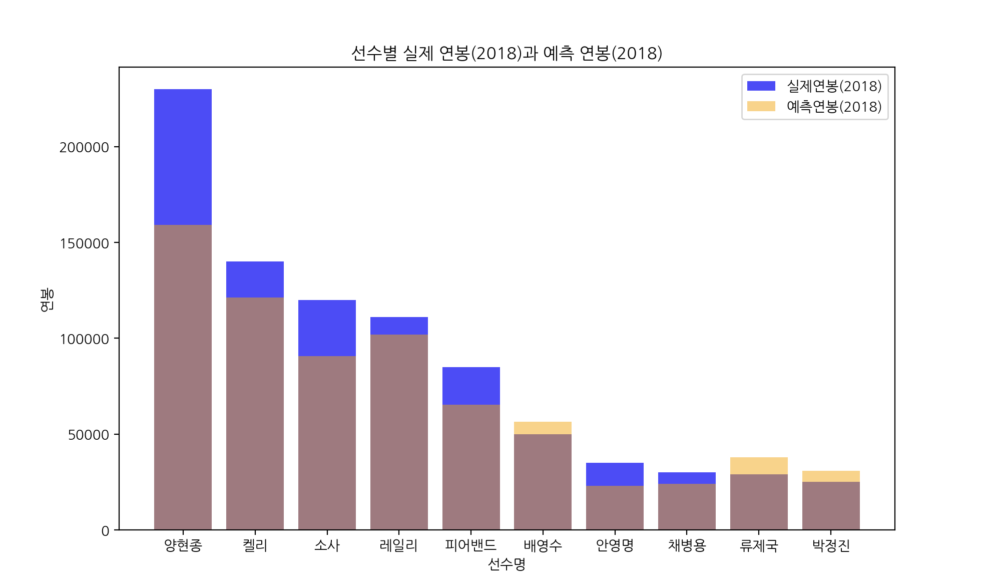
비슷한듯 다른듯...그런것 같습니다
