Faster R-CNN
Abstract
Sota를 달성한 object detection network들은 객체 위치를 예측하기 위해 region proposal 알고리즘에 의존한다. SPPnet과 Fast R-CNN 같은 발전으로 네트워크 실행시간을 단축시킬 수 있었지만, region proposal을 계산에서 병목현상이 발생하였다.
따라서, 전체 이미지의 detection 네트워크와 전체 이미지의 convolution 특징을 공유하여 비용이 거의 들지 않는 RPN이라는 네트워크를 제안한다.
RPN은 각 위치에서 객체의 경계와 객체성 점수를 동시에 예측하는 fully convolution convoultion 네트워크이며, 높은 퀄리티의 region proposal을 생성하기 위해서 end-to-end로 학습된다.
따라서, RPN은 Fast R-CNN의 convolution 특징과 RPN의 특징을 공유함으로써 single 네트워크로 병합함으로, 최근에 인기있는 attention 매커니즘을 통해 통합된 네트워크가 바라보아야할 위치를 지시한다.
Introduction
기존의 R-CNN과 Fast R-CNN의 region proposal은 Selective search를 사용하여 CPU상에서 생성되었기 때문에 속도가 느렸다. 이를 GPU에서 활용하기 위해 RPN을 사용하여 region proposal을 추출하였고, 하나의 네트워크로 연결하여 end-to-end로 학습할 수 있는 Faster R-CNN이 등장하였다.
Fast R-CNN은 같은 region 기반 detector에서 나온 convolutional feature map들이 바로 region proposal 생성에 사용될 수 있다는 것을 관찰 했으며, 이를 통해 end-to-end로 학습할 수 있었다고 한다.
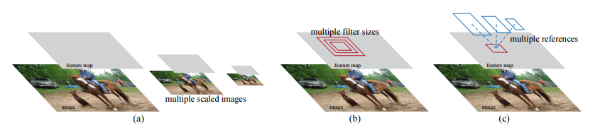
RPN은 큰 범위와 측면 비율을 통해 region proposal을 효율적으로 예측하도록 설계되었다. 피라미드 형태의 새로운 앵커 박스를 도입하여 multi-scale과 측면 비율들을 참조하여 사용하였고 이는 훈련 및 테스트에서 우수한 성능을 냈다고 한다.
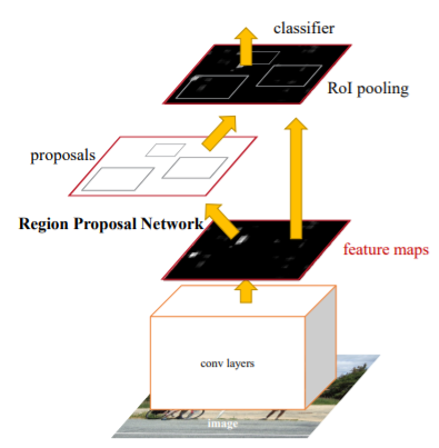
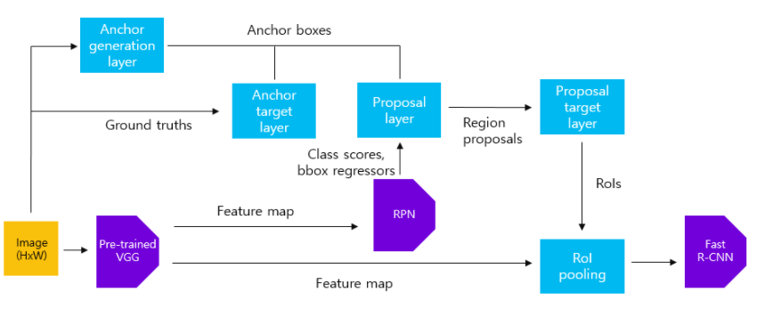
Faster R-CNN의 구조는 아래 그림과 같이 RPN + Fast R-CNN의 구조와 같다
Architecture
-
input
- input은 scale에 상관없이 이미지를 받으며, output으로는 사각형의 객체 지역과, 각 위치 안에 객체가 있는지 나타내는 점수를 출력한다
-
Feature Etraction
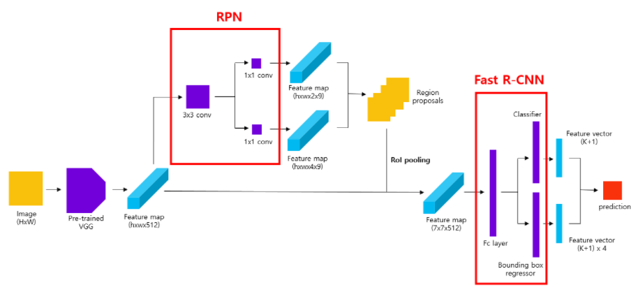
- pretrained model을 사용하여 feature map 생성
-
RPN
- input으로 pretrained model에서 뽑은 feature map을 넣는다.
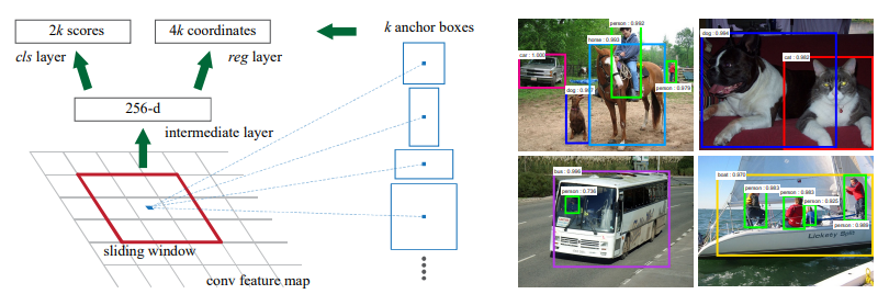
- feature map 위에서 sliding window방법을 사용(3 x 3 filter) 하여 intermediate layer생성.
- 이때 크기를 유지하기 위해 padding 추가
- intermediate layer의 각 위치마다 k개의 anchor box 생성 ( 논문에서는 3개의 scale x 3개의 aspect ratio 사용하여 총 9 개의 anchor box 생성)
- cls layer , reg layer의 채널을 맞춰주기 위해 1x1 conv 사용
- cls layer에서는 k개 anchor box 안에 객체가 있는지 없는지에 대한 2(object 여부) x k(anchor box 개수) channel 출력
- reg layer는 k개의 anchor box의 좌표(높이,너비, 중앙 x,y좌표)의 4 x 9의 channel 출력
-
Classification layer
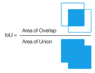
- IOU를 사용해서 각 anchor box와 ground truth box가 overlab되는 정도를 비교
- IOU가 0.7이상이거나 가장 크면 possitive , 0.3 보다 적으면 negative, 이외에는 0으로 두어 학습할 데이터를 줄인다
-
이후 NMS방법에 따라 class 별 상위 N개의 region proposal를 추출
- NMS
- 주로 중복되는 Bounding box를 제거하기 위해 사용된다.
- 예측한 box들 중 score에 따라 상위 boxes를 추출
- 추출한 box와 다른 box들을 1:1로 비교해가며 IoU가 기준(Threshold)보다 높은 경우 같은 물체를 가리키고 있다고 판단하여 제거
- 이를 반복하며 최종적으로 class별 score에 따라 상위 N개의 box가 추출된다.
- NMS
-
Regressor layer
- 상위 N개의 anchor box의 4개 좌표와 ground truth의 4개 좌표를 비교하여 bounding box를 출력
-
ROI pooling
- RPN을 지나면 서로 다른 region proposal이 나오는데 이를 ROI pooling을 통해 동일한 크기의 vector를 생성
- 이후 동일한 크기의 region proposal를 Faster R-CNN에 전달
-
Loss
- : classification의 Log Loss
- : bbox regression의 smooth L1 loss
- : mini-batch size
- : anchor 위치의 수
- : Predicted probability of anchor
- : Ground Truth label (1 or 0)
- : Predicted Bounding box
- : Ground-truth box
- : blancing parameter(defualt =10)
Faster R-CNN 학습 과정
-
pre-train된 VGG16 모델에 원본 이미지를 넣어 feature map생성 (sub sampling ratio 1/16)
- input : 800 x 800 x 3 sized image
- Process : pretrained VGG16
- output : 50 x 50 x 512 feature map
-
원본이미지에서 sub sampling ration만큼의 grid cell이 생성되고 각 위치에서 anchor box를 생성 (Anchor generation layer)
- input : 800 x 800 x 3 sized image
- Process : generate anchor box
- output : 50 x 50 x 9 feature map ( 50 x 50 의 grid cell에서 각 9개의 anchor box)
-
RPN을 학습시키기 위한 anchor sample 구성(anchor target layer)
-
IOU ≥ 0.7 : Positive(1)
-
IOU ≤ 0.3 : Negative(-1)
-
0.3 < IOU < 0.7 : 0
-
Positive,Negative 비율이 1:1이 되도록 Sampling ( positive 256, negative 256)
-
만약 Positive의 개수가 부족하다면 Zero padding을 하거나 IoU 값이 가장 높은 box를 positive로 사용
-
input : 50 x 50 x 9 anchor boxes, ground truth boxes
-
process : select anchor samples
-
output : positive/negative anchor boxes
-
-
RPN에 VGG16에서 나온 feature map을 input으로 넣고 3x3 conv를 거친 후 각각의 1x1 conv를 통해 class score와 bounding box regressor를 추출
- input : 50 x 50 x 512 sized image
- Process : RPN
- output : class score (50 x 50 x 2 x 9) , bbox regressors(50 x 50 x 4 x 9) feature map
-
RPN에서 얻은 class score, bounding box regressor를 NMS 방법으로 class별 상위 N개의 region proposal 추출(Proposal layer)
- input : 22500(50 x 50 x 9) anchor boxes , class score and bbox regressors feature map
- Process : select region proposal with NMS
- output : 상위 N개의 region proposal
-
Fast R-CNN을 학습하기 위한 region proposal Sampling(Proposal target layer)
-
추출한 상위 N개의 region proposal과 GT의 IOU를 계산.
-
IOU ≥ 0.5 : Positive
-
0.1 ≤ IOU < 0.5 : Negative
-
input : 상위 N개의 region proposal, ground truth boxes
-
Process : labeling region proposal
-
output : positive/negative region proposals
-
-
맨 처음 원본이미지를 VGG16 모델에 넣어 나온 feature map과 6을 통해 얻은 region proposals들을 사용하여 ROI pooling 수행(ROI pooling)
- input : 50 x 50 x 512 feature map, positive/negative region proposals
- Process : ROI pooling
- output : 7 x 7 x 512 feature map
-
Loss에 따른 Fast R-CNN 학습 (Fast R-CNN)
-
입력받은 feature map을 fc layer에 입력해서 4096 크기의 feature vector를 얻는다
-
feature vector를 Classifier와 bbox regressor에 입력
-
출력된 결과를 loss를 이용해 학습
-
input : 7 x 7 x 512 feature map
-
Process : feature extraction, Classifier, regressior, train Fast R-CNN by loss
-
output : loss
-
Alternating training
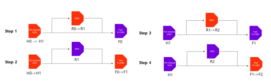
- RPN 학습
- Imagenet pre-trained model을 불러와서 featuer map을 생성하고 원본 이미지에서 anchor boxes를 추출한다.
- 이들을 통해 RPN을 학습하며 동시에 pre-trained model도 학습
- Fast R-CNN 학습
- RPN으로 추출된 region proposal들을 활용해 Fast R-CNN학습
- 이 단계도 동시에 pre-trained model도 학습
- 다시 RPN 학습
- 앞서 1,2번에서 학습한 RPN과 Fast R-CNN을 불러와서 RPN에 해당하는 부분만 fine tuning 하여 학습한다.
- 이 때 pre-trained model은 freeze 하여 학습하지 않는다.
- 다시 Fast R-CNN학습
- 3번에서 추출한 region proposal을 활용하여 Fast R-CNN을 학습한다.
- 이 때 RPN과 pre-trained model은 freeze 하여 학습하지 않는다.
Experiment
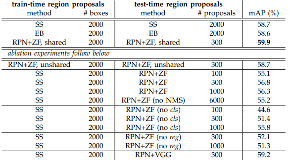
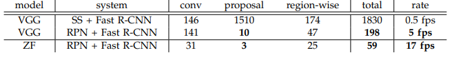
- PASCAL VOC 2007 test set으로 실험한 결과 RPN을 사용했을 때가 mAP가 높은 것을 볼 수 있다.
- 또한, SS보다 속도면에서 훨씬 성능이 좋은 것을 볼 수 있다.
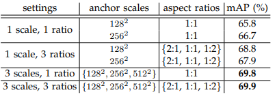
- anchor box를 생성할 때 3 scales , 3 ratios 를 사용한 것이 mAP가 가장 높게 나타났다.
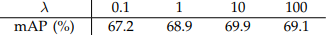
- 람다는 10을 사용했을 때 mAP가 가장 높게 나타났기에 10을 사용
장점 : selective search 대신 RPN을 제안하여 GPU에서 수행되게 하여 속도를 빠르게함
단점 : Real time Detector가 되기엔 역부족?
