이번주에는 alexnet, vggnet, resnet 이라는 세개의 cnn 아키텍쳐를 비교해보고, 코드까지 작성하고 실행해보았습니다.
1. 데이터
데이터는 torchvision의 CIFAR10 데이터를 사용했다.
a. 모델 훈련 코드
from tqdm.notebook import tqdm

def training_model(model, data_loader, epochs):
  since = time.time() # 총 소요 시간 계산을 위해시작 시간을 기록

  best_model_wts = copy.deepcopy(model.state_dict())  # 모든 epoch에서 학습 된 모델 중 best model의 가중치를 저장하는 변수
  best_acc = 0

  for epoch in range(epochs):
    avg_cost = 0

    for phase in ['train', 'val']:  # train mode와 validation mode 순서로 진행
        if phase == 'train':
            model.train()  # model을 training mode로
        else:
            model.eval()   # model을 validation mode로

        for X, Y in tqdm(data_loader[phase]):
            X, Y = X.to(device), Y.to(device)

            optimizer.zero_grad()   # 지난 iteration에서 계산했던 기울기 초기화

            with torch.set_grad_enabled(phase == 'train'):  # training mode에서는 gradient를 기억하여 가중치를 수정해야 함
                                                            # validation mode에서는 가중치를 수정하지 않으므로 필요 없음
                hypothesis = model(X)   # 순전파 과정으로 예측값 도출
                cost = criterion(hypothesis, Y)   # 예측값과 실제값을 비교한 loss

                if phase == 'train':
                    cost.backward()   # 역전파, 기울기 계산
                    optimizer.step()   # optimizer로 가중치 갱신
                    avg_cost += cost / total_batch[phase]

                else: # validation에서는 역전파로 가중치를 학습할 필요 없음
                    prediction = model(X)   # 학습한 모델로 test 데이터의 예측값 도출(각 숫자에 해당할 확률)
                    prediction = prediction.to(device)
                    correct_prediction = torch.argmax(prediction, 1) == Y   # 모든 확률 중에서 가장 큰 확률을 가진 숫자를 예측값으로 지정하고 이를 실제값과 비교
                    global accuracy
                    accuracy = correct_prediction.float().mean().item()   # 정확도 계산

        if phase == 'train':
            print('[Epoch: {:>4}] train cost = {:.4f}'.format(epoch + 1, avg_cost)) # training 과정에서 각 epoch 마다의 cost 출력
        else:
            print('val Accuracy = {:.4f}', accuracy)  # validation 과정에서 각 epoch에서 학습된 모델의 성능 출력
            print('='*100)

        if phase == 'val' and accuracy > best_acc:  # 이번 epoch에서 만들어진 모델이 이전에 만들어진 모델보다 더 성능이 좋을 경우, best accuracy을 수정
            best_acc = accuracy
            best_model_wts = copy.deepcopy(model.state_dict())

  training_time = time.time() - since   # 학습 경과 시간
  print('total training time for {} epochs: {:.0f}m {:.0f}s'.format(epochs, training_time//60, training_time%60))
  print('Best val Accuracy: {:.4f}'.format(best_acc))

  model.load_state_dict(best_model_wts)
  return model  # best model 반환
b. Data Augmentation
데이터의 양을 늘리기 위해 원본에 각종 변환을 적용하여 개수를 증강시키는 기법
# Data Augmentation
transform = transforms.Compose([
  transforms.Resize(256),
  transforms.RandomCrop(227),
  transforms.ToTensor(),
  transforms.Normalize((0.5, 0.5, 0.5), (0.5, 0.5, 0.5))  #3채널(R,G,B) 데이터의 평균과 분산을 0.5로 설정
])
c. 데이터 준비
# 예시속은 CIFAR-10 dataset을 사용했습니다.

batch_size = 64

cifar_train = datasets.CIFAR10('~/.data', download=True, train=True, transform=transform)
train_loader = torch.utils.data.DataLoader(cifar_train, batch_size=batch_size, shuffle=True)  #batch_size는 원하는 크기로 변경 가능.
                                                                                              #단, 2의 제곱수로 하고 test_loader의 batch_size도 동일한 수로 변경할 것.

cifar_test = datasets.CIFAR10('~/.data', download=True, train=False, transform=transform)
test_loader = torch.utils.data.DataLoader(cifar_test, batch_size=batch_size, shuffle=True)

data_loaders = {'train' : train_loader, 'val': test_loader}
total_batch = {'train' : len(train_loader), 'val': len(test_loader)}

classes = ('plane', 'car', 'bird', 'cat', 'deer', 'dog', 'frog', 'horse', 'ship', 'truck')

# 클래스 총 10개 지정

from torchvision import utils
import matplotlib.pyplot as plt
import numpy as np

dataiter = iter(train_loader)   # iter함수로 iteration 객체 가져오기
images, labels = next(dataiter)
2. CNN 모델
a. AlextNet
- CNN Network layer의 목적은 더 깊은 네트워크를 만들면서 (레이어 수를 늘려 정확도 상승), 성능/학습능력 을 높여가는 것 (파라미터 수를 줄여 처리 속도 감소)입니다.
- AlexNet의 문제
- 고해상도 이미지에 대규모로 CNN을 적용하기에는 여전히 많은 연산량이 소모됩니다.
- 적은 데이터셋을 가져 과적합의 문제를 수반합니다.
- AlexNet의 핵심 설명
- 학습 최적화를 위해 ReLU 활성화 함수를 사용하고, 2개의 GPU를 병렬로 두고 사용합니다.
- 오버피팅의 문제를 해결하기 위해 Data Augmentation, Dropout의 방법을 사용합니다.
- CNN이 본격적으로 많이 사용된 계기가 된 모델이나 비교적 구조가 간단해서 최근에 많이 사 용되는 모델은 아닙니다.
AlexNet 코드 구현
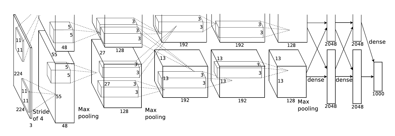
첫번째 레이어(컨볼루션 레이어)
- 96개의 11 x 11 x 3 사이즈 필터커널, stride=4, padding=0
- 55 x 55 x 96 사이즈 특성맵
- ReLU 함수로 활성화
- 3 x 3 overlapping max pooling, stride=2
- local response normalization
→ Result: 27 x 27 x 96 size의 특성맵
# 1st Conv layer
nn.Conv2d(in_channels=3,
	out_channels=96,
	kernel_size=11,
	padding=0,
	stride=4
),
nn.ReLU(inplace=True),
nn.MaxPool2d(kernel_size=3, stride=2),  # overlap pooling, 55->27
nn.LocalResponseNorm(size=5, alpha=0.0001, beta=0.75, k=2),- Q. LocalResponseNorm이란? ReLU 활성화 함수 사용 시, 양수의 경우 값을 그대로 출력하기 때문에 특징이 너무 뚜렷하여 값이 너무 큰 경우에 주변의 영향을 주는 것을 막기 위해 사용됩니다.
→ local response norm 이후 값이 작아집니다.
두번째 레이어(컨볼루션 레이어)
- 256개의 5 x 5 x 48 커널, stride=1, padding=2
- 27 x 27 x 256 사이즈 특성맵
- ReLU 함수로 활성화
- 3 x 3 overlapping max pooling, stride 2
- local response normalization
→ Result: 13 x 13 x 256 size의 특성맵
# 2nd Conv layer
nn.Conv2d(96, 256, 5, padding=2, stride=1),  # 27->27
nn.ReLU(inplace=True),
nn.LocalResponseNorm(size=5, alpha=0.0001, beta=0.75, k=2),
nn.MaxPool2d(kernel_size=3, stride=2),  # 27->13
세번째 레이어(컨볼루션 레이어)
- 384개의 3 x 3 x 256 커널, stride=1, padding=1
- 13 x 13 x 384 사이즈 특성맵
- ReLU 함수로 활성화
→ Result: 13 x 13 x 384 size의 특성맵
# 3rd Conv layer
nn.Conv2d(256, 384, 3, padding=1, stride=1),  # 13->13
nn.ReLU(inplace=True),
네번째 레이어(컨볼루션 레이어)
- 384개의 3 x 3 x 192 커널, stride=1, padding=1
- 13 x 13 x 384 사이즈 특성맵
- ReLU 함수로 활성화
→ Result: 13 x 13 x 384 size의 특성맵
# 4th Conv layer
nn.Conv2d(384, 384, 3, padding=1, stride=1),  # 13->13
nn.ReLU(inplace=True),
다섯번째 레이어(컨볼루션 레이어)
- 256개의 3 x 3 x 192 커널, stride=1 padding=1
- 13 x 13 x 256 사이즈 특성맵
- ReLU 함수로 활성화
- 3 x 3 overlapping max pooling, stride=2
→ Result: 6 x 6 x 256 size의 특성맵
# 5th Conv layer
nn.Conv2d(384, 256, 3, padding=1, stride = 1),  # 13->13
nn.ReLU(inplace=True),
nn.MaxPool2d(kernel_size=3, stride=2),  # 13->6
여섯번째 레이어(Fully connected layer):
- 6 x 6 x 256 특성맵을 flatten → 6 x 6 x 256 = 9216 차원의 벡터
- 그것을 여섯번째 레이어의 4096개의 뉴런과 fully connect
- 그 결과를 ReLU 함수로 활성화
# 1st Fully connected layer
nn.Linear(in_features=(256 * 6 * 6), out_features=4096),
nn.ReLU(inplace=True),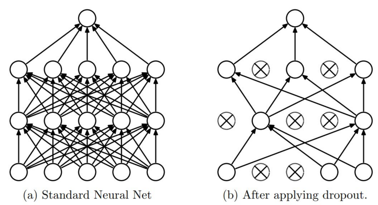
nn.Dropout(p=0.5),- Q. Dropout이란? 신경망의 뉴런을 부분적으로 생략하여 모델의 오버피팅을 해결해주기 위한 방법입니다.
일곱번째 레이어(Fully connected layer):
- 4096개의 뉴런으로 구성
- 전 단계의 4096개 뉴런과 fully connected
- 출력 값은 ReLU 함수로 활성화
nn.Linear(in_features=4096, out_features=4096),
nn.ReLU(inplace=True),
nn.Dropout(p=0.5),
여덟번째 레이어(Fully connected layer):
- 1000개(경우에 따라 다르므로 num_classes로 지정해준다)의 뉴런으로 구성
- 전 단계의 4096개 뉴런과 fully connected
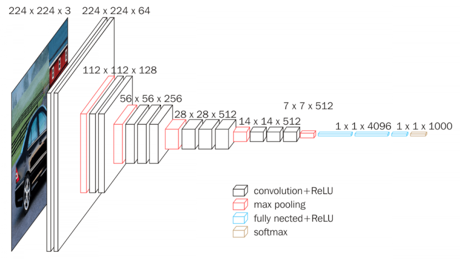
nn.Linear(in_features=4096, out_features=num_classes),b. VGGNet
- 기존 모델의 문제 개선
- AlexNet의 8-layer보다 2배 이상 더 깊은 층을 쌓으면서 학습하여 Alexnet의 에러율을 절반으로 줄였습니다.
- VGG 모델 이전에는 비교적 큰 Receptive Field를 갖는 11x11필터나 7x7 필터를 사용했습니다.
- VGG 핵심 설명
- 신경망 깊이(레이어 수)가 깊어질수록 이미지 분류 성능이 높아짐을 보여주었습니다.
- 3x3 작은 필터를 고정적으로 사용하여 연산과정에서 비선형성을 증가시키고, 학습 파라미터 수를 감소시켜 성능을 높였습니다.
- 2014년 VGG 모델은 ILSVRC 대회에 출현하여 GoogLeNet에 뒤이어 2번째로 좋은 성능을 보였습니다. 간단한 구조이지만 비교적 복잡한 GoogleNet과 거의 비슷한 성능을 보여준다는 점에서 신경망 깊이의 유효성을 증명했다고 할 수 있습니다.
representation depth is beneficial for the classification accuracy, and that state-of-the-art performance on the ImageNet challenge dataset can be achieved using a conventional ConvNet architecture with substantially increased depth.
VGGNet 코드 구현
- 사전에 쓰이는 함수
def conv_2_block(in_features, out_features):
  net = nn.Sequential(
    nn.Conv2d(in_features, out_features, kernel_size = 3, padding = 1),
    nn.ReLU(),
    nn.Conv2d(out_features, out_features, kernel_size = 3, padding = 1),
    nn.ReLU(),
    nn.MaxPool2d(2, 2)
	 )
  return net
def conv_3_block(in_features, out_features):
net = nn.Sequential(
nn.Conv2d(in_features, out_features, kernel_size = 3, padding = 1),
nn.ReLU(),
nn.Conv2d(out_features, out_features, kernel_size = 3, padding = 1),
nn.ReLU(),
nn.Conv2d(out_features, out_features, kernel_size = 3, padding = 1),
nn.ReLU(),
nn.MaxPool2d(2, 2)
)
return netdef vgg_block(num_convs, in_channels, out_channels):
layers = []
for _ in range(num_convs):
layers.append(nn.Conv2d(in_channels, out_channels, kernel_size = 3, padding = 1))
layers.append(nn.ReLU(inplace = True))
in_channels = out_channels
layers.append(nn.MaxPool2d(kernel_size = 2, stride = 2))
return nn.Sequential(*layers)1층
-
1차 Conv2d
64개의 3 x 3 x 3 필터커널, padding=1, stride=1
→ 결과적으로 64장의 224 x 224 특성맵(224 x 224 x 64)들이 생성됩니다.ReLU 함수 적용
-
2차 Conv2d
****64개의 3 x 3 x 64 필터커널, padding=1, stride=1
→ 결과적으로 64장의 224 x 224 특성맵들(224 x 224 x 64)이 생성됩니다.ReLU 함수 적용
-
Max pooling을 사용하여 특성맵의 사이즈를 112 X 112 X 64로 줄입니다.
conv_2_block(3, 64), # 3->642층
-
1차 Conv2d
256개의 3 x 3 x 128 필터커널, padding=1, stride=1
→ 결과적으로 256장의 56 x 56 특성맵(56 x 56 x 256)들이 생성됩니다.ReLU 함수 적용
-
2차 Conv2d
256개의 3 x 3 x 256 필터커널, padding=1, stride=1
→ 결과적으로 256장의 56 x 56특성맵들(56 x 56 x 256)이 생성됩니다.ReLU 함수 적용
-
3차 Conv2d (2차와 동일)
256개의 3 x 3 x 256 필터커널, padding=1, stride=1
→ 결과적으로 256장의 56 x 56특성맵들(56 x 56 x 256)이 생성됩니다.ReLU 함수 적용
-
Max pooling을 사용하여 특성맵의 사이즈를 28 X 28 X 256로 줄입니다.
conv_3_block(128, 256), # 128->2563층
-
1차 Conv2d
512개의 3 x 3 x 256 필터커널, padding=1, stride=1
→ 결과적으로 512장의 28 x 28 특성맵(28 x 28 x 512)들이 생성됩니다.ReLU 함수 적용
-
2차 Conv2d
512개의 3 x 3 x 512 필터커널, padding=1, stride=1
→ 결과적으로 512장의 28 x 28특성맵들(28 x 28 512)이 생성됩니다.ReLU 함수 적용
-
3차 Conv2d (2차와 동일)
512개의 3 x 3 x 512 필터커널, padding=1, stride=1
→ 결과적으로 512장의 28 x 28특성맵들(28 x 28 512)이 생성됩니다.ReLU 함수 적용
-
Max pooling을 사용하여 특성맵의 사이즈를 14 X 14 X 512로 줄입니다.
conv_3_block(256, 512), # 256->5124층
-
1차 Conv2d
512개의 3 x 3 x 512 필터커널, padding=1, stride=1
→ 결과적으로 512장의 14 x 14 특성맵(14 x 14 x 512)들이 생성됩니다.ReLU 함수 적용
-
2차 Conv2d
512개의 3 x 3 x 512 필터커널, padding=1, stride=1
→ 결과적으로 512장의 14 x 14 특성맵(14 x 14 x 512)들이 생성됩니다.ReLU 함수 적용
-
3차 Conv2d (2차와 동일)
512개의 3 x 3 x 512 필터커널, padding=1, stride=1
→ 결과적으로 512장의 14 x 14 특성맵(14 x 14 x 512)들이 생성됩니다.ReLU 함수 적용
-
Max pooling을 사용하여 특성맵의 사이즈를 7 X 7 X 512로 줄입니다.
conv_3_block(512, 512), # 512->5125층(FC 1차)
- 7 x 7 x 512의 특성맵을 flatten 해줍니다.
- 결과적으로 7 x 7 x 512 = 25088개의 뉴런이 됩니다.
- fc1차의 4096개의 뉴런과 fully connected 됩니다.
- 훈련시 dropout이 적용됩니다.
nn.Linear(512*4*4, 4096),
nn.ReLU(inplace=True),
nn.Dropout(),
6층(FC 2차)
- 4096개의 뉴런으로 구성해줍니다.
- fc1차의 4096개의 뉴런과 fully connected 됩니다.
- 훈련시 dropout이 적용됩니다.
nn.Linear(4096, 1000),
nn.ReLU(inplace=True),
nn.Dropout(),
7층(FC 3차)
- 1000개의 뉴런(해다 코드에서는 num_classes로 일반화)으로 구성됩니다.
- fc2층의 4096개의 뉴런과 fully connected됩니다.
- (원래 출력값들은 softmax 함수로 활성화됩니다.)
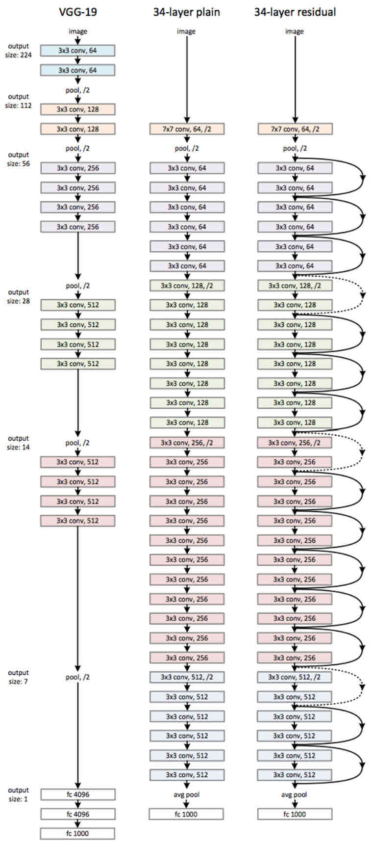
nn.Linear(1000, num_classes),c. ResNet
- 기존 모델의 문제점
- 레이어를 깊게 쌓을수록 train/test 에러율이 높아졌습니다.
- 기존의 매핑인 H(x) 를 그대로 학습시켰을 때 최적화와, 학습의 수렴이 어려운 문제가 존재했습니다.
- ResNet의 핵심 설명
- 기존의 매핑인 H(x) 를 F(x) +x 로 식을 변환시켜 잔차 블록인 F(x) 만 학습시키는 방식을 취했습니다.
- 배치 정규화를 통해 학습 속도 감소, 가중치 초기화에 대한 민감도를 감소 시켰습니다.
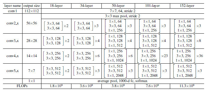
- 50 layer 이상의 레이어를 쌓을 경우 Bottleneck 구조를 취해 파라미터 연산을 줄였습니다.
- 잔차 블록을 학습함으로써 신경망이 152 레이어까지 더 깊은 층을 가지면서도, 학습 난이도나 파라미터 연산을 줄이며 오차율을 감소시킬 수 있었습니다.
- Image classification 문제 뿐만 아니라 Object Dectection, Image Segmentation 문제 등 다양한 비전 문제에서 좋은 성능을 보였습니다.
ResNet 코드 구현
- 사전에 사용되는 함수
def conv_block_1(in_features, out_features, stride=1):
    net = nn.Sequential(
        nn.Conv2d(in_features, out_features, kernel_size=1, stride = stride),
        nn.BatchNorm2d(out_features),
        nn.ReLU(),
    )
    return net
def conv_block_3(in_features, out_features, stride=1):
net = nn.Sequential(
nn.Conv2d(in_features, out_features, kernel_size = 3, stride = stride, padding = 1),
nn.BatchNorm2d(out_features),
nn.ReLU(),
)
return net- Q. BatchNorm2d이란? (배치 정규화) BatchNorm2d 함수는 배치 정규화를 위한 함수입니다. layer 가 깊은 딥러닝 모델은 복잡하고 오버피팅이 일어나기 쉽습니다. 특히, 데이터 전처리 방식에 따라 모델의 결과는 큰 차이를 가집니다. 배치 정규화가 나오게 된 배경을 이해하기 위해서는 Covariance Shift 를 이해해야 합니다 .
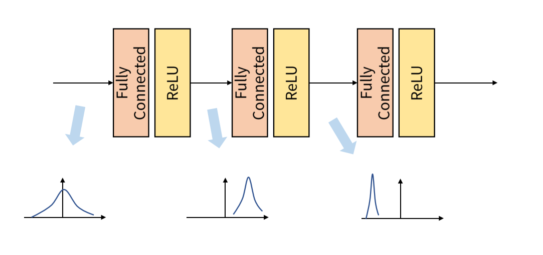 Covariance Shift 란 이전 레이어의 파라미터 변화로 인하여 현재 레이어의 입력의 분포가 바뀌는 현상입니다.
Internal Covariance Shift 는 레이어를 통과할 때마다 Covariance Shift 가 일어나면서 입력의 분포가 약간씩 변하는 현상입니다. 위 그림과 같이 layer를 거칠 때마다 데이터의 분포가 달라지는 것입니다.
Batch Normalization 은 이 Internal Covariance Shift 문제를 해결하기 위해 나온 것인데, 학습 과정에서 배치 단위 별로 데이터가 서로 다른 분포를 가지더라도 배치들의 평균과 분산을 이용해 정규화하는 것을 의미합니다. 배치별로 다른 분포에 있는 데이터를 Zero mean gaussian 형태로 만듦으로써 평균은 0, 표준편차는 1로 분포를 동일하게 맞춰줍니다.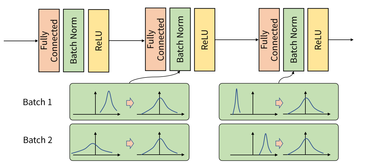
배치 정규화를 적용하면 Internal Covariance Shift 현상을 해결하고자 진행하는 가중치 초기화와 learning rate를 감소 과정에서 자유로워질 수 있습니다.
배치 정규화의 또다른 이점으로는 Regularization Effect 가 있습니다. 배치 정규화를 진행할 때, 배치에 들어가는 평균과 분산에 지속적으로 변화를 주는 과정에서 가중치 업데이트에도 영향을 주어 가중치가 큰 방향으로만 학습되지 않기 때문에 Regularization Effect 를 얻을 수 있습니다. 이는 궁극적으로 오버피팅될 확률을 낮춰주게 됩니다.
- Bottleneck (병목현상)
class BottleNeck(nn.Module):
    def __init__(self, in_features, mid_features, out_features, down=False):
        super(BottleNeck, self).__init__()
        self.down=down

        # feature map 크기가 감소하는 경우
        if self.down:
            self.layer = nn.Sequential(
              conv_block_1(in_features, mid_features, stride=2),
              conv_block_3(mid_features, mid_features, stride=1),
              conv_block_1(mid_features, out_features, stride=1),
            )
            self.downsample = nn.Conv2d(in_features, out_features, kernel_size=1, stride=2)

        # feature map의 크기가 유지되는 경우
        else:
            self.layer = nn.Sequential(
                conv_block_1(in_features, mid_features, stride=1),
                conv_block_3(mid_features, mid_features, stride=1),
                conv_block_1(mid_features, out_features, stride=1),
            )

        self.dim_equalizer = nn.Conv2d(in_features, out_features, kernel_size=1)

    def forward(self, x):
        if self.down:
            downsample = self.downsample(x)
            output = self.layer(x)
            output = output + downsample
        else:
            output = self.layer(x)
            if x.size() is not output.size():
                x = self.dim_equalizer(x)
            output = output + x
return output- Resnet 함수
class ResNet(nn.Module):
    def __init__(self, num_classes=10):
        super(ResNet, self).__init__()

        self.layer_1 = nn.Sequential(
            nn.Conv2d(3,64,kernel_size = 7, stride = 2, padding=3),
            nn.ReLU(),
            nn.MaxPool2d(3,2,1),
        )
        self.layer_2 = nn.Sequential(
            BottleNeck(64,64,256),
            BottleNeck(256,64,256),
            BottleNeck(256,64,256,down=True),
        )
        self.layer_3 = nn.Sequential(
            BottleNeck(256,128,512),
            BottleNeck(512,128,512),
            BottleNeck(512,128,512),
            BottleNeck(512,128,512,down=True),
        )
        self.layer_4 = nn.Sequential(
            BottleNeck(512,256,1024),
            BottleNeck(1024,256,1024),
            BottleNeck(1024,256,1024),
            BottleNeck(1024,256,1024),
            BottleNeck(1024,256,1024),
            BottleNeck(1024,256,1024,down=True),
        )
        self.layer_5 = nn.Sequential(
            BottleNeck(1024,512,2048),
            BottleNeck(2048,512,2048),
            BottleNeck(2048,512,2048),
        )
        self.avgpool = nn.AvgPool2d(1,1)
        self.fc_layer = nn.Linear(2048,num_classes)

    def forward(self, x):
        output = self.layer_1(x)
        output = self.layer_2(output)
        output = self.layer_3(output)
        output = self.layer_4(output)
        output = self.layer_5(output)
        output = self.avgpool(output)
        output = output.view(batch_size,-1)
        output = self.fc_layer(output)

        return output