이번 글에서는 양방향 LSTM을 이용해 품사 태깅을 해 볼 것이다. 양방향을 쓰게되면 문장의 처음과 끝 문맥을 잘 반영할 수 있게 된다.

패키지를 다운받아주자.

Packages

import nltk
import numpy as np
%matplotlib inline
import matplotlib.pyplot as plt
from tensorflow.keras.preprocessing.text import Tokenizer
from tensorflow.keras.preprocessing.sequence import pad_sequences
from tensorflow.keras.utils import to_categorical
from sklearn.model_selection import train_test_split

NLTK에서는 토큰화와 품사 태깅이 완료된 데이터를 불러올 수 있다.

nltk.download('treebank')
tagged_sentences = nltk.corpus.treebank.tagged_sents()

Data Preprocessing

데이터를 tagged_sentences안에 저장하였다.
길이와 내용을 출력해서 전체 문장의 길이와 내용을 확인해보자.

len(tagged_sentences)

print(tagged_sentences)

토큰화가 완료된 단어와 그에 맞는 품사 태깅이 같이 나온다.
이 둘을 분리해주기 위해서 먼저 빈 테이블을 만들어주고, zip을 이용해 둘을 분리하여 각각 테이블에 넣어주면 된다.

sentences = []
pos_tags = []

for tagged_sentence in tagged_sentences:
  sentence, tag_info = zip(*tagged_sentence)
  sentences.append(list(sentence))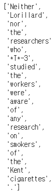
  pos_tags.append(list(tag_info))

sentences의 출력 결과:

pos_tags의 출력 결과:

단어와 품사태깅이 분리되었다.

이번에는 케라스 토크나이즈를 이용해서 정수 인코딩을 해보자.

Encoding

문장 데이터와 레이블 모두에게 정수 인코딩을 해 주어야 하기 때문에 한번에 함수로 만들어서 진행한다.

def tokenize(samples):
  tokenizer = Tokenizer()
  tokenizer.fit_on_texts(samples)
  return tokenizer

각각 토큰화를 해 준다.

src_token = tokenize(sentences)
tar_token = tokenize(pos_tags)

각각의 크기를 확인해보자.

vocab_size = len(src_token.word_index) + 1
tag_size = len(tar_token.word_index) + 1
print(vocab_size)
print(tag_size)

11388개의 단어집합과 47개의 태그가 존재한다.
인코딩 해 주자.
문장은 X_train안에, 태그는 y_train안에 넣었다.

X_train = src_token.texts_to_sequences(sentences)
y_train = tar_token.texts_to_sequences(pos_tags)

출력해서 확인해보자.

print(X_train[:2])

print(y_train[:2])

이제 패딩을 해 보자.

Padding

패딩을 하기 전에 max_len을 정해줘야한다.
전체길이를 그래프로 한번에 확인해보자.

plt.hist([len(s) for s in X_train], bins=50)
plt.xlabel('length of samples')
plt.ylabel('number of samples')
plt.show()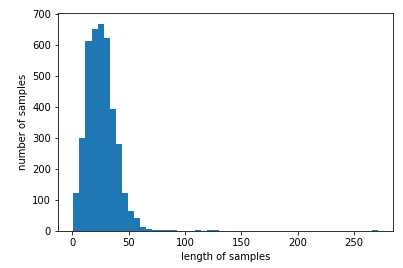

최대 길이를 150정도로 하면 괜찮을 것 같다.
설정해주고 패딩해주자.

max_len = 150
X_train = pad_sequences(X_train, padding='post', maxlen = max_len)
y_train = pad_sequences(y_train, padding='post', maxlen = max_len)

모든 전처리가 끝났으니 테스트 샘플과 훈련 샘플로 나눠줘야 한다.

Split Sample

X_train, X_test, y_train, y_test = train_test_split(X_train, y_train, test_size=.2, random_state=777)

이 한줄로 쉽게 분리할 수 있다.
test_size=0.2는 전체 데이터 셋의 20%를 test (validation) 셋으로 지정하겠다는 의미다.
random_state는 세트를 섞을 때 해당 int 값을 보고 섞으며, 하이퍼 파라미터를 튜닝시 이 값을 고정해두고 튜닝해야 매번 데이터셋이 변경되는 것을 방지할 수 있다. 그냥 아무 숫자값이나 집어넣어도 무방하다.

One-hot Encoding

이제 해당하는 태깅 정보에 대해서 원-핫 인코딩을 해준다.

y_train = to_categorical(y_train, num_classes=tag_size)
y_test = to_categorical(y_test, num_classes=tag_size)

모델을 구축해보자.

Build Model

Packages

from keras.models import Sequential
from keras.layers import Dense, LSTM, InputLayer, Bidirectional, TimeDistributed, Embedding
from tensorflow.keras.optimizers import Adam

이제 모델을 만들어보자.

model = Sequential()
model.add(Embedding(vocab_size, 128, input_length=max_len, mask_zero=True))
model.add(Bidirectional(LSTM(256, return_sequences=True)))
model.add(TimeDistributed(Dense(tag_size, activation=('softmax'))))
model.compile(optimizer=Adam(0.001), loss='categorical_crossentropy', metrics=['acc'])

val_data를 추가해서 학습해준다.

history=model.fit(X_train, y_train, batch_size=128, epochs=10, validation_data=(X_test,y_test))

평가해보자.

model.evaluate(X_test,y_test)[1]

93%정도가 나왔다.

마지막으로 train세트와 val세트를 그래프로 확인해보자.

epochs = range(1, len(history.history['acc']) + 1)
plt.plot(epochs, history.history['acc'])
plt.plot(epochs, history.history['val_acc'])
plt.title('model accuracy')
plt.ylabel('accuracy')
plt.xlabel('epochs')
plt.legend(['train', 'test'], loc='lower right')
plt.show()

epochs = range(1, len(history.history['loss']) + 1)
plt.plot(epochs, history.history['loss'])
plt.plot(epochs, history.history['val_loss'])
plt.title('model loss')
plt.ylabel('loss')
plt.xlabel('epochs')
plt.legend(['train', 'test'], loc='upper right')
plt.show()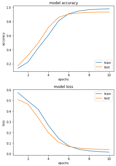

여기서 설명을 마치겠다.