
라이브러리 가져오기
import torch
import torch.nn as nn
기초
데이터를 만들어보자. torch.randn을 이용하여 random numbers from a normal distribution with mean 0 and variance 1 을 가져온다.
preds = torch.randn(5)
print(preds)
tensor([-0.6459, 0.8710, -0.4781, 0.6219, -0.3734])
매번 모델을 돌릴때마다 랜덤한 값을 가지고 실험할 수 없으니,
랜덤 결과를 맞춰주는 방법이 필요하다.
torch.manual_seed(0)를 가지고 랜덤시드를 맞춰준다.
torch.manual_seed(0)
preds = torch.randn(5)
print(preds)
아마 이 코드를 돌리면 모든 사람들의 랜덤한 결과가 같을 것이다.
tensor([ 1.5410, -0.2934, -2.1788, 0.5684, -1.0845])
만약 랜덤시드가 다르면 다른 결과값이 나온다.
이번에는 0 대신 2023을 넣어보자.
torch.manual_seed(0)
preds = torch.randn(5)
print(preds)
tensor([-1.2075, 0.5493, -0.3856, 0.6910, -0.7424])
다른 값이 나오지만 랜덤시드를 2023으로 설정한 모든 사람들에게는 같은 결과가 출력된다.
이번에는 2차원으로 실습해보자.
2*3 텐서로 확장시킨다.
torch.manual_seed(2023)
preds = torch.randn(2, 3)
print(preds)
tensor([[-1.2075, 0.5493, -0.3856],
[ 0.6910, -0.7424, 0.1570]])
이렇게 2차원 텐서가 만들어졌다.
우리는 예측값으로 0부터 1 사이의 확률이 나와야 하므로 pytorch.rand를 사용해서 2*3텐서의 랜덤 데이터를 만들어보자.
torch.manual_seed(2023)
preds = torch.rand(2, 3)
print(preds)
tensor([[0.4290, 0.7201, 0.9481],
[0.4797, 0.5414, 0.9906]])
예측값 생성하기
이번에는 같은 코드지만, BATCH_SIZE와 N_CLASS라는 변수를 정해주고 거기에 맞는 크기의 랜덤 데이터를 만들어보자.
torch.manual_seed(2023)

BATCH_SIZE = 4
N_CLASSES = 7

preds = torch.rand(BATCH_SIZE, N_CLASSES)
print(preds)
tensor([[0.4290, 0.7201, 0.9481, 0.4797, 0.5414, 0.9906, 0.4086],
[0.2183, 0.1834, 0.2852, 0.7813, 0.1048, 0.6550, 0.8375],
[0.1823, 0.5239, 0.2432, 0.9644, 0.5034, 0.0320, 0.8316],
[0.3807, 0.3539, 0.2114, 0.9839, 0.6632, 0.7001, 0.0155]])
다음으로 처리해야 할 문제는,
preds가 모델이 예측한 확률이면 가로로 모든 값을 더했을 때 1이 나와야 한다.
다 더했을 때 1이 나오려면, 방금 출력한 각각의 값에다가 가로별로 쭉 더한 값을 나눠주면 되지 않을까?
아마도 preds = preds / preds.sum(axis = 1)라는 라인을 넣으면 될 것 같다.
하지만 여기서 텐서가 맞지 않는 현상이 발생한다.
(4,7) 나누기 (4, )는 일어나지 않는다. 따라서 (4, )에 대해 shape을 맞춰줘야 하므로,
preds = preds / preds.sum(axis = 1).reshape(BATCH_SIZE, -1) 이 라인이 들어가야 한다.
torch.manual_seed(2023)

BATCH_SIZE = 4
N_CLASSES = 7

preds = torch.rand(BATCH_SIZE, N_CLASSES)
print(preds)
preds = preds / preds.sum(axis = 1).reshape(BATCH_SIZE, -1)
print(preds)
print(preds.sum(axis=1))
tensor([[0.4290, 0.7201, 0.9481, 0.4797, 0.5414, 0.9906, 0.4086],
[0.2183, 0.1834, 0.2852, 0.7813, 0.1048, 0.6550, 0.8375],
[0.1823, 0.5239, 0.2432, 0.9644, 0.5034, 0.0320, 0.8316],
[0.3807, 0.3539, 0.2114, 0.9839, 0.6632, 0.7001, 0.0155]])
tensor([[0.0950, 0.1594, 0.2099, 0.1062, 0.1198, 0.2193, 0.0904],
[0.0712, 0.0598, 0.0930, 0.2549, 0.0342, 0.2137, 0.2732],
[0.0556, 0.1597, 0.0741, 0.2940, 0.1534, 0.0098, 0.2535],
[0.1151, 0.1069, 0.0639, 0.2974, 0.2004, 0.2116, 0.0047]])
tensor([1.0000, 1.0000, 1.0000, 1.0000])
처음 출력된 텐서는 이전 텐서이고
다음으로 출력된 텐서는 가로 합을 1로 맞춘 텐서이다.
마지막 줄에서는 가로 합이 1인 것을 확인하는 코드를 출력하였다.
정답값 생성하기(원-핫 벡터)
다시 처음으로 돌아와서 랜덤시드를 설정해준 후, zero들로 텐서 사이즈를 맞춰보자.
torch.manual_seed(2023)

labels = torch.zeros(size=(BATCH_SIZE, N_CLASSES))
print("init")
print(labels, '\n')
init
tensor([[0., 0., 0., 0., 0., 0., 0.],
[0., 0., 0., 0., 0., 0., 0.],
[0., 0., 0., 0., 0., 0., 0.],
[0., 0., 0., 0., 0., 0., 0.]])
공간을 만들어 준 셈이다.
그 다음에 우리는 torch.randint을 이용하여 클래스 개수에 맞게 랜덤 클래스를 뽑아보자.
labels_ = torch.randint(low = 0, high =N_CLASSES, size=(BATCH_SIZE, ))
print("labels")
print(labels_, '\n')
labels
tensor([6, 2, 4, 3])
이 뜻은 4개의 이미지가 각각 레이블6, 레이블2, 레이블4, 레이블3 이라는 것을 의미한다.
이 레이블들을 원-핫 인코딩을 통해서 바꿔보자.
torch.arange를 사용한다.
labels[torch.arange(BATCH_SIZE), labels_] = 1
print("one-hot encoding")
print(labels)
one-hot encoding
tensor([[0., 0., 0., 0., 0., 0., 1.],
[0., 0., 1., 0., 0., 0., 0.],
[0., 0., 0., 0., 1., 0., 0.],
[0., 0., 0., 1., 0., 0., 0.]])
이런 결과가 나오는데, 아까 처음 이미지의 레이블은 6이었다.
여기 출력 중 첫 번째 줄을 보면 [0., 0., 0., 0., 0., 0., 1.] 이렇게 되어있는데, 바로 6번째에 1이 들어와있다.
(0부터 세기 때문에 따지자면 7번째이지만, 레이블로 봤을 때에는 6이다.)
이와 같은 방법으로 원-핫 인코딩으로 봤을 때, 각각의 사진들의 레이블들을 확인할 수 있다.
Cross Entropy (1)
One-hot encoding 안되어있는 상태
import torch
import torch.nn as nn

torch.manual_seed(2023)

BATCH_SIZE = 4
N_CLASSES = 7

preds = torch.rand(BATCH_SIZE, N_CLASSES) # 모델의 예측(클래스별 확률)이라고 가정
preds = preds / preds.sum(axis=1).reshape(-1, 1) # (4, 7) ~ (4, 1): broadcasting

labels = torch.randint(low=0, high=N_CLASSES, size=(BATCH_SIZE, ))
print(preds)
print(labels)

preds = preds[torch.arange(BATCH_SIZE), labels]
ce_loss = -torch.mean(torch.log(preds))
print(ce_loss)
Cross Entropy (2)
One-hot encoding + sum 이용
import torch
import torch.nn as nn

torch.manual_seed(2023)

BATCH_SIZE = 4
N_CLASSES = 7

preds = torch.rand(BATCH_SIZE, N_CLASSES) # 모델의 예측(클래스별 확률)이라고 가정
preds = preds / preds.sum(axis=1).reshape(-1, 1) # (4, 7) ~ (4, 1): broadcasting

labels = torch.zeros(size=(BATCH_SIZE, N_CLASSES))
labels[torch.arange(BATCH_SIZE), torch.randint(low=0, high=N_CLASSES, size=(BATCH_SIZE, ))] = 1

print(preds)
print(labels, '\n')

cross_entropy = -torch.mean(torch.log((preds * labels).sum(axis=1)))
print(preds * labels)
print((preds * labels).sum(axis=1))
print(cross_entropy, '\n')
Cross Entropy (3)
One-hot encoding + indexing 이용
import torch
import torch.nn as nn

torch.manual_seed(2023)

BATCH_SIZE = 4
N_CLASSES = 7

preds = torch.rand(BATCH_SIZE, N_CLASSES) # 모델의 예측(클래스별 확률)이라고 가정
preds = preds / preds.sum(axis=1).reshape(-1, 1) # (4, 7) ~ (4, 1): broadcasting

labels = torch.zeros(size=(BATCH_SIZE, N_CLASSES))
labels[torch.arange(BATCH_SIZE), torch.randint(low=0, high=N_CLASSES, size=(BATCH_SIZE, ))] = 1

print(preds)
print(labels, '\n')

row_indices, col_indices = torch.where(labels == 1)
cross_entropy = -torch.mean(torch.log(preds[row_indices, col_indices]))
print(cross_entropy)
CrossEntropy 모듈 사용하기
import torch.nn as nn

BATCH_SIZE = 4
N_CLASSES = 7

preds = torch.rand(BATCH_SIZE, N_CLASSES) # 모델의 예측(클래스별 확률)이라고 가정
preds = preds / preds.sum(axis=1).reshape(-1, 1) # (4, 7) ~ (4, 1): broadcasting
print(preds)

labels = torch.zeros(size=(BATCH_SIZE, N_CLASSES))
labels = torch.randint(low=0, high=N_CLASSES, size=(BATCH_SIZE, ))
print(labels)

loss_fn = nn.CrossEntropyLoss()

loss = loss_fn(preds, labels)
print(loss)
loss_fn = nn.CrossEntropyLoss()를 사용하여 쉽게 loss를 구할 수 있다.
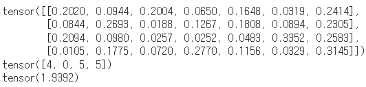
처음으로 출력되는 텐서는 예측값이고
두번째로 출력되는 건 실제값이다.
마지막으로 출력되는 loss는 이를 모두 합산하여 배치의 평균 손실을 계산한 값이다.
이 값은 신경망의 성능을 평가하는 지표로 사용되며, 신경망의 가중치를 업데이트하는 데에도 사용된다.
이 값이 작을수록 모델의 예측이 실제 레이블에 가깝다는 것을 의미한다.
다음 글에서는 softmax에 대해서 설명한다.