C1W3A1 Planar Data Classification with One Hidden Layer
은닉층이 1개인 신경망을 만들어보자!
준비
# Package imports
import numpy as np
import copy
import matplotlib.pyplot as plt
from testCases_v2 import *
from public_tests import *
import sklearn
import sklearn.datasets
import sklearn.linear_model
from planar_utils import plot_decision_boundary, sigmoid, load_planar_dataset, load_extra_datasets

%matplotlib inline

%load_ext autoreload
%autoreload 2
# Load the dataset
X, Y = load_planar_dataset()- a numpy-array (matrix) X that contains your features (x1, x2)
- a numpy-array (vector) Y that contains your labels (red:0, blue:1).
두 행렬 X, Y를 얻었다.
# Visualize the data:
plt.scatter(X[0, :], X[1, :], c=Y, s=40, cmap=plt.cm.Spectral);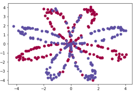
matplotlib를 사용하여 데이터를 시각화하면 위와 같은 이미지로 나타난다.
shape_X = X.shape
shape_Y = Y.shape
m = X.shape[1];
m은 training example의 개수이다.
Simple Logistic Regression
본격적으로 신경망을 만들기 전에, 이 문제에 대해 로지스틱 회귀는 어떻게 동작하는지 살펴보자
# Train the logistic regression classifier
clf = sklearn.linear_model.LogisticRegressionCV();
clf.fit(X.T, Y.T);
sklearn의 빌트인함수를 사용하여, 로지스틱 회귀 분류기를 학습시킨다.
# Plot the decision boundary for logistic regression
plot_decision_boundary(lambda x: clf.predict(x), X, Y)
plt.title("Logistic Regression")

# Print accuracy
LR_predictions = clf.predict(X.T)
print ('Accuracy of logistic regression: %d ' % float((np.dot(Y,LR_predictions) + np.dot(1-Y,1-LR_predictions))/float(Y.size)*100) +
       '% ' + "(percentage of correctly labelled datapoints)")
Accuracy of logistic regression: 47 %
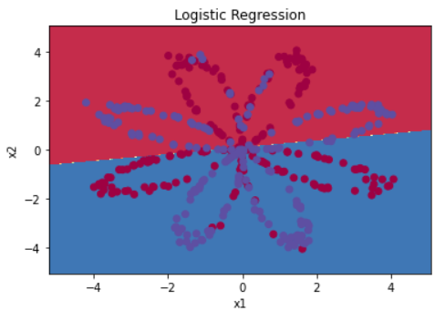
데이터들이 선형으로 분류될 수 없기 때문에, 로지스틱 회귀는 좋지 않은 성능을 보인다.
Neural Network Model
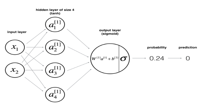
위 모델처럼 은닉층이 1개인 신경망을 만들 것이다.
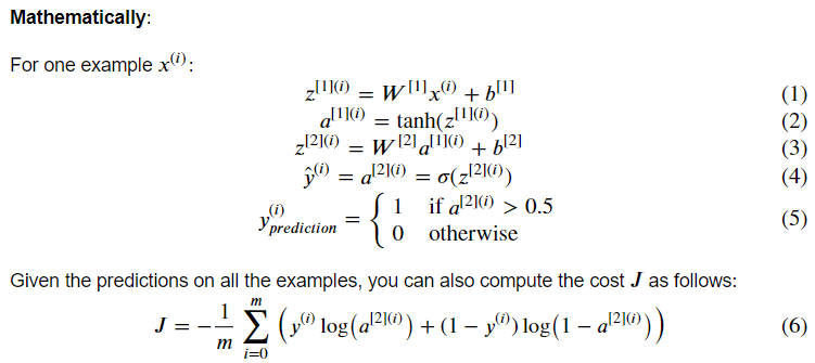
이를 식으로 나타내면
✅신경망을 만드는 일반적인 방법론
1. 신경망 구조 정의 (# of input units, # of hidden units, etc)
2. 모델 파라미터 초기화
3. Loop: FP, loss 계산, BP(gradient 계산), update parameters(경사하강법)
로지스틱 회귀 모델을 만들때와 마찬가지로, 1-3 부분을 각각 구현한 뒤 nn_model()로 합칠 것이다.
1. Defining the neural network structure
def layer_sizes(X, Y):
	n_x = X.shape[0]
    n_y = Y.shape[0]
    n_h = 4

return (n_x, n_h, n_y)- n_x: 입력층의 크기
- n_h: 은닉층의 크기 (여기서만 4로 하드코딩)
- n_y: 출력층의 크기
2. Initialize the model's parameters
def initialize_parameters(n_x, n_h, n_y):
	W1 = np.random.randn(n_h, n_x) * 0.01
    b1 = np.zeros((n_h, 1))
    W2 = np.random.randn(n_y, n_h) * 0.01
    b2 = np.zeros((n_y, 1))

    parameters = {"W1": W1,
                  "b1": b1,
                  "W2": W2,
                  "b2": b2}

return parameters- W1: weight matrix of shape (n_h, n_x)
- b1: bias vector of shape (n_h, 1)
- W2: weight matrix of shape (n_y, n_h)
- b2: bias vector of shape (n_y, 1)
매개변수들의 크기를 알맞게 설정하자
3. The Loop
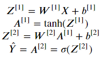
위 식들을 사용해 FP를 구현하자
def forward_propagation(X, parameters):
	# Retrieve each parameter from the dictionary "parameters"
	W1 = parameters["W1"]
    b1 = parameters["b1"]
    W2 = parameters["W2"]
    b2 = parameters["b2"]

    # Implement Forward Propagation to calculate A2 (probabilities)
    Z1 = np.dot(W1, X) + b1
    A1 = np.tanh(Z1)
    Z2 = np.dot(W2, A1) + b2
    A2 = sigmoid(Z2)

    ssert(A2.shape == (1, X.shape[1]))

    cache = {"Z1": Z1,
             "A1": A1,
             "Z2": Z2,
             "A2": A2}

    return A2, cache
4. Compute the Cost
비용함수 식은 다음과 같다:
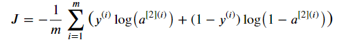
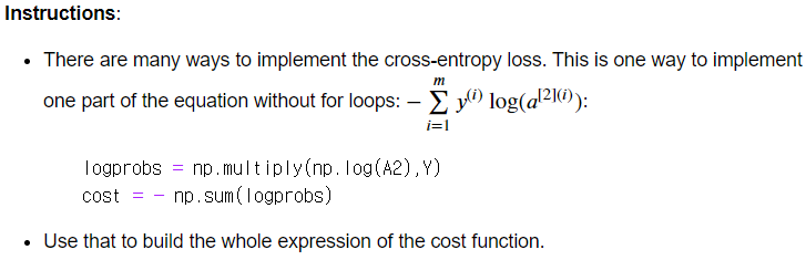
위 식을 이용해 비용함수 J의 값을 계산해보자
def compute_cost(A2, Y):
	m = Y.shape[1] # number of examples

    # Compute the cross-entropy cost
	logprobs = np.multiply(Y, np.log(A2)) + np.multiply((1-Y), np.log(1-A2))
    cost = np.sum(logprobs) / -m

    cost = float(np.squeeze(cost))  # makes sure cost is the dimension we expect.
                                    # E.g., turns [[17]] into 17

    return cost
조금 복잡해 보이지만 다음을 참고해서 코드를 짜면 된다.
5. Implement Backward Propagation
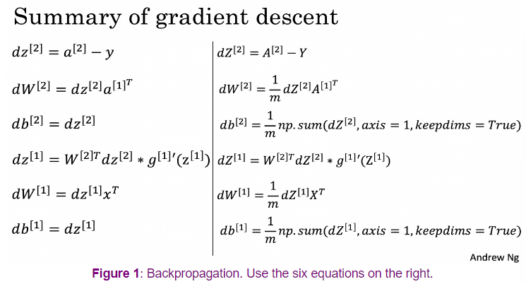
오른쪽 6개의 식을 사용하여 BP를 구현하자
def backward_propagation(parameters, cache, X, Y):
"""
    Implement the backward propagation using the instructions above.

    Arguments:
    parameters -- python dictionary containing our parameters
    cache -- a dictionary containing "Z1", "A1", "Z2" and "A2".
    X -- input data of shape (2, number of examples)
    Y -- "true" labels vector of shape (1, number of examples)

    Returns:
    grads -- python dictionary containing your gradients with respect to different parameters
    """
	m = X.shape[1]

    # First, retrieve W1 and W2 from the dictionary "parameters".
    W1 = parameters["W1"]
    W2 = parameters["W2"]

    # Retrieve also A1 and A2 from dictionary "cache".
    A1 = cache["A1"]
    A2 = cache["A2"]

    # Backward propagation: calculate dW1, db1, dW2, db2.
    dZ2 = A2 - Y
    dW2 = np.dot(dZ2, A1.T) / m
    db2 = np.sum(dZ2, axis=1, keepdims=True) / m
    dZ1 = np.dot(W2.T, dZ2) * (1 - np.power(A1, 2))
    dW1 = np.dot(dZ1, X.T) / m
    db1 = np.sum(dZ1, axis=1, keepdims=True) / m

    grads = {"dW1": dW1,
             "db1": db1,
             "dW2": dW2,
             "db2": db2}

    return grads
6. Update Parameters
경사하강법을 사용하여 매개변수를 업데이트하자

def update_parameters(parameters, grads, learning_rate = 1.2):
	"""
    Updates parameters using the gradient descent update rule given above

    Arguments:
    parameters -- python dictionary containing your parameters
    grads -- python dictionary containing your gradients

    Returns:
    parameters -- python dictionary containing your updated parameters
    """

    # Retrieve a copy of each parameter from the dictionary "parameters". Use copy.deepcopy(...) for W1 and W2
    W1 = parameters["W1"]
    b1 = parameters["b1"]
    W2 = parameters["W2"]
    b2 = parameters["b2"]

    # Retrieve each gradient from the dictionary "grads"
    dW1 = grads["dW1"]
    db1 = grads["db1"]
    dW2 = grads["dW2"]
    db2 = grads["db2"]

    # Update rule for each parameter
    W1 = W1 - learning_rate * dW1
    b1 = b1 - learning_rate * db1
    W2 = W2 - learning_rate * dW2
    b2 = b2 - learning_rate * db2

    parameters = {"W1": W1,
                  "b1": b1,
                  "W2": W2,
                  "b2": b2}

    return parameters
Integration
구현한 함수들을 알맞게 사용하여 nn_model()에 신경망 모델을 만들자
def nn_model(X, Y, n_h, num_iterations = 10000, print_cost=False):
	"""
    Arguments:
    X -- dataset of shape (2, number of examples)
    Y -- labels of shape (1, number of examples)
    n_h -- size of the hidden layer
    num_iterations -- Number of iterations in gradient descent loop
    print_cost -- if True, print the cost every 1000 iterations

    Returns:
    parameters -- parameters learnt by the model. They can then be used to predict.
    """

    np.random.seed(3)
    n_x = layer_sizes(X, Y)[0]
    n_y = layer_sizes(X, Y)[2]

    # Initialize parameters
    parameters = initialize_parameters(n_x, n_h, n_y)

    # Loop (gradient descent)
    for i in range(0, num_iterations):
    	#FP
    	A2, cache = forward_propagation(X, parameters)
        #Cost function
        cost = compute_cost(A2, Y)
        #BP
        grads = backward_propagation(parameters, cache, X, Y)
        # Gradient descent parameter update
        parameters = update_parameters(parameters, grads)

        # Print the cost every 1000 iterations
        if print_cost and i % 1000 == 0:
            print ("Cost after iteration %i: %f" %(i, cost))

    return parameters
Test the Model
1. Predict
def predict(parameters, X):
	"""
    Using the learned parameters, predicts a class for each example in X

    Arguments:
    parameters -- python dictionary containing your parameters
    X -- input data of size (n_x, m)

    Returns
    predictions -- vector of predictions of our model (red: 0 / blue: 1)
    """

    # Computes probabilities using forward propagation, and classifies to 0/1 using 0.5 as the threshold.
     A2, cache = forward_propagation(X, parameters)
    predictions = (A2 > 0.5)

    return predictions
활성화값이 0.5가 넘으면 예측값을 1로, 0.5 이하이면 예측값을 0으로 설정한다.
2. Test the Model on the Planar Dataset
구현한 신경망이 어떻게 동작하는지 확인해보자
# Build a model with a n_h-dimensional hidden layer
parameters = nn_model(X, Y, n_h = 4, num_iterations = 10000, print_cost=True)

# Plot the decision boundary
plot_decision_boundary(lambda x: predict(parameters, x.T), X, Y)
plt.title("Decision Boundary for hidden layer size " + str(4))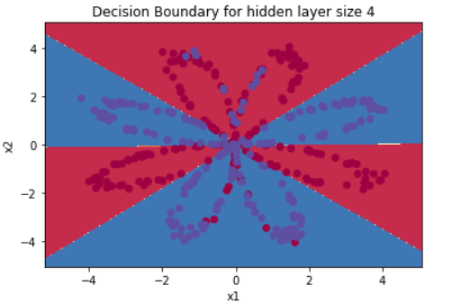
훌륭하다
# Print accuracy
predictions = predict(parameters, X)
print ('Accuracy: %d' % float((np.dot(Y, predictions.T) + np.dot(1 - Y, 1 - predictions.T)) / float(Y.size) * 100) + '%')
Accuracy: 90%
잘 동작한다!
Tuning hidden layer size
# This may take about 2 minutes to run

plt.figure(figsize=(16, 32))
#hidden_layer_sizes = [1, 2, 3, 4, 5]

# you can try with different hidden layer sizes
# but make sure before you submit the assignment it is set as "hidden_layer_sizes = [1, 2, 3, 4, 5]"
hidden_layer_sizes = [1, 2, 3, 4, 5, 20, 50]

for i, n_h in enumerate(hidden_layer_sizes):
    plt.subplot(5, 2, i+1)
    plt.title('Hidden Layer of size %d' % n_h)
    parameters = nn_model(X, Y, n_h, num_iterations = 5000)
    plot_decision_boundary(lambda x: predict(parameters, x.T), X, Y)
    predictions = predict(parameters, X)
    accuracy = float((np.dot(Y,predictions.T) + np.dot(1 - Y, 1 - predictions.T)) / float(Y.size)*100)
    print ("Accuracy for {} hidden units: {} %".format(n_h, accuracy))
Accuracy for 1 hidden units: 67.5 %
Accuracy for 2 hidden units: 67.25 %
Accuracy for 3 hidden units: 90.75 %
Accuracy for 4 hidden units: 90.5 %
Accuracy for 5 hidden units: 91.25 %
Accuracy for 20 hidden units: 91.0 %
Accuracy for 50 hidden units: 90.5 %
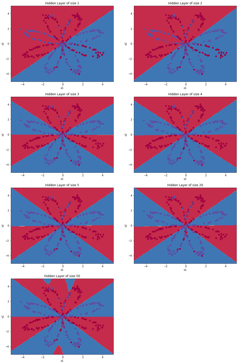
은닉유닛의 개수가 더 많은 큰 모델은 훈련세트를 더 잘 맞춘다. 그러나 너무 크면 데이터를 과적합한다. 여기서 가장 좋은 은닉층의 크기는 n_h=5 근처로 보인다 (훈련세트를 잘 맞추면서도 과적합이 발생하지 않음).
나중에 정규화를 배우고 나서 n_h=50 이상의 아주 큰 모델도 사용해보자
