C1W2A2 Logistic Regression with a Neural Network

로지스틱 회귀를 사용해 고양이 분류기를 만들어보자!

준비

먼저 필요한 패키지들을 임포트해준다.

import numpy as np
import copy
import matplotlib.pyplot as plt
import h5py
import scipy
from PIL import Image
from scipy import ndimage
from lr_utils import load_dataset
from public_tests import *

%matplotlib inline
%load_ext autoreload
%autoreload 2

훈련세트와 테스트세트가 포함된 data.h5가 주어진다. 아래 코드로 데이터를 불러온다. 이미지 데이터셋 x 뒤에 _orig를 붙인 이유는 해당 데이터를 전처리할 것이기 때문이다. (y는 전처리가 필요없다)

# Loading the data (cat/non-cat)
train_set_x_orig, train_set_y, test_set_x_orig, test_set_y, classes = load_dataset()

아래 코드는 훈련세트에서 해당 인덱스를 가진 이미지와 레이블을 출력해준다.

# Example of a picture
index = 25
plt.imshow(train_set_x_orig[index])
print ("y = " + str(train_set_y[:, index]) + ", it's a '" + classes[np.squeeze(train_set_y[:, index])].decode("utf-8") +  "' picture.")

훈련샘플의 개수, 테스트샘플의 개수, 훈련할 이미지의 가로=세로 길이를 얻는다.

m_train = train_set_x_orig.shape[0]
m_test = test_set_x_orig.shape[0]
num_px = train_set_x_orig.shape[1]

훈련세트와 테스트세트를 reshape한다.
크기가 (num_px, num_px, 3)이던 이미지를 (num_px num_px 3, 1)로 납작하게 만든다.

train_set_x_flatten = train_set_x_orig.reshape(train_set_x_orig.shape[0], -1).T
test_set_x_flatten = test_set_x_orig.reshape(test_set_x_orig.shape[0], -1).T

데이터를 "standardize"

train_set_x = train_set_x_flatten / 255.
test_set_x = test_set_x_flatten / 255.

이것으로 데이터세트의 전처리를 마쳤다.

---

이제 본격적으로 모델을 만들어보자. 신경망을 구축하는 단계는 다음과 같다:
1. 모델 구조를 짠다(입력 특성의 개수 등)
2. 모델 parameter를 초기화한다
3. Loop : FP(loss 계산), BP(gradient 계산), Update parameters(경사 하강법)

1-3 부분을 각각 만들고 model() 함수로 합쳐보자

Helper functions

Sigmoid

def sigmoid(z):
	s = 1 / (1 + np.exp(z))
	return s

Initializing parameters

def initialize_with_zeros(dim):
	w = np.zeros((dim, 1))
    b = 0.0
    return w, b

w (dim $\times$ 1)차원 벡터, b는 float
0으로 초기화된 매개변수들을 반환한다.

FP & BP

def propagate(w, b, X, Y):
	m = X.shape[1]
    
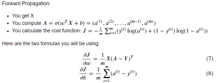
    # FORWARD PROPAGATION (FROM X TO COST)
    A = sigmoid(np.dot(w.T, X) + b) 
    cost = np.sum(Y * np.log(A) + (1-Y) * np.log(1-A)) / -m
    
    # BACKWARD PROPAGATION (TO FIND GRAD)
    dw = np.dot(X, (A-Y).T) / m
    db = np.sum(A-Y) / m
    
    cost = np.squeeze(np.array(cost))

    grads = {"dw": dw,
             "db": db}
    
    return grads, cost

비용함수와 gradient를 계산한다.

Optimization

def optimize(w, b, X, Y, num_iterations=100, learning_rate=0.009, print_cost=False):
	w = copy.deepcopy(w)
    b = copy.deepcopy(b)
    
    costs = []
    
    for i in range(num_iterations):
      	# Cost and gradient calculation 
    	grads, cost = propagate(w, b, X, Y) 
        
         # Retrieve derivatives from grads
        dw = grads["dw"]
        db = grads["db"]
        
        # update rule 
        w = w - learning_rate * dw
        b = b - learning_rate * db
        
        # Record the costs
        if i % 100 == 0:
            costs.append(cost)
        
            # Print the cost every 100 training iterations
            if print_cost:
                print ("Cost after iteration %i: %f" %(i, cost))
    
    params = {"w": w,
              "b": b}
    
    grads = {"dw": dw,
             "db": db}
    
    return params, grads, costs

Predict

이전 함수에서 학습한 w와 b를 사용해 레이블을 예측한다.

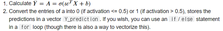
def predict(w, b, X):
	m = X.shape[1]
    Y_prediction = np.zeros((1, m))
    w = w.reshape(X.shape[0], 1)
    
    # Compute vector "A" predicting the probabilities of a cat being present in the picture
    A = sigmoid(np.dot(w.T, X) + b)
    
    for i in range(A.shape[1]):
    	# Convert probabilities A[0,i] to actual predictions p[0,i]
        if A[0, i] > 0.5:
            Y_prediction[0, i] = 1;
        else:
            Y_prediction[0, i] = 0;
            
   	return Y_prediction

여기까지 정의한 함수들:
w,b 초기화
w,b 학습을 위해 반복적으로 loss 최적화 (cost와 gradient 계산, parameters 업데이트)
학습된 w,b로 레이블 예측

Merge

model

• Y_prediction_test for your predictions on the test set
• Y_prediction_train for your predictions on the train set
• parameters, grads, costs for the outputs of optimize()

def model(X_train, Y_train, X_test, Y_test, num_iterations=2000, 
		  learning_rate=0.5, print_cost=False):
	# initialize parameters with zeros
    w, b = initialize_with_zeros(X_train.shape[0])
     
    # Gradient descent 
    params, grads, costs = optimize(w, b, X_train, Y_train, num_iterations, learning_rate, print_cost)
    
    # Retrieve parameters w and b from dictionary "params"
    w = params["w"]
    b = params["b"]
    
    # Predict test/train set examples
    Y_prediction_test = predict(w, b, X_test)
    Y_prediction_train = predict(w, b, X_train)

    # Print train/test Errors
    if print_cost:
        print("train accuracy: {} %".format(100 - np.mean(np.abs(Y_prediction_train - Y_train)) * 100))
        print("test accuracy: {} %".format(100 - np.mean(np.abs(Y_prediction_test - Y_test)) * 100))

    
    d = {"costs": costs,
         "Y_prediction_test": Y_prediction_test, 
         "Y_prediction_train" : Y_prediction_train, 
         "w" : w, 
         "b" : b,
         "learning_rate" : learning_rate,
         "num_iterations": num_iterations}
    
    return d

위와 같이 함수를 정의한 후, 아래 코드를 실행시켜 모델을 훈련시킨다.

logistic_regression_model = model(train_set_x, train_set_y, test_set_x, test_set_y, num_iterations=2000, learning_rate=0.005, print_cost=True)

train accuracy: 99.04306220095694 %
test accuracy: 70.0 %

# Example of a picture that was wrongly classified.
index = 10
plt.imshow(test_set_x[:, index].reshape((num_px, num_px, 3)))
print ("y = " + str(test_set_y[0,index]) + ", you predicted that it is a \"" + classes[int(logistic_regression_model['Y_prediction_test'][0,index])].decode("utf-8") +  "\" picture.")

위 코드는 테스트세트에서 해당 인덱스를 가진 이미지와 예측된 레이블을 출력한다.

# Plot learning curve (with costs)
costs = np.squeeze(logistic_regression_model['costs'])
plt.plot(costs)
plt.ylabel('cost')
plt.xlabel('iterations (per hundreds)')
plt.title("Learning rate =" + str(logistic_regression_model["learning_rate"]))
plt.show()

위 코드를 실행시키면, 아래와 같은 출력을 얻을 수 있다.

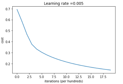
비용이 점차 감소하는 모습이다. 파라미터가 학습되고 있음을 보여준다.
반복횟수를 늘리면, 훈련세트 정확도는 증가할 것이지만 테스트세트 정확도는 낮아질 것이다(overfitting).

---

분석

Choice of learning rate

learning_rates = [0.01, 0.001, 0.0001]
models = {}

for lr in learning_rates:
    print ("Training a model with learning rate: " + str(lr))
    models[str(lr)] = model(train_set_x, train_set_y, test_set_x, test_set_y, num_iterations=1500, learning_rate=lr, print_cost=False)
    print ('\n' + "-------------------------------------------------------" + '\n')

for lr in learning_rates:
    plt.plot(np.squeeze(models[str(lr)]["costs"]), label=str(models[str(lr)]["learning_rate"]))

plt.ylabel('cost')
plt.xlabel('iterations (hundreds)')

legend = plt.legend(loc='upper center', shadow=True)
frame = legend.get_frame()
frame.set_facecolor('0.90')
plt.show()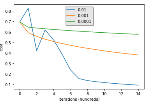

학습률은 얼마나 급속히 파라미터를 업데이트할지를 결정한다. 학습률이 너무 작으면, 최적의 값을 찾기 위해 너무 많은 반복이 필요하다. 너무 크면, 최적의 값을 overshoot하게 될 것이다. 따라서 학습률을 잘 선택해야 한다.