System Model And Problem Formulation

System model은 다음의 두 level로 구성된다: Semantic level & Transmission level. (아래의 그림을 보자)

Fig. 1. The framework of proposed DeepSC.

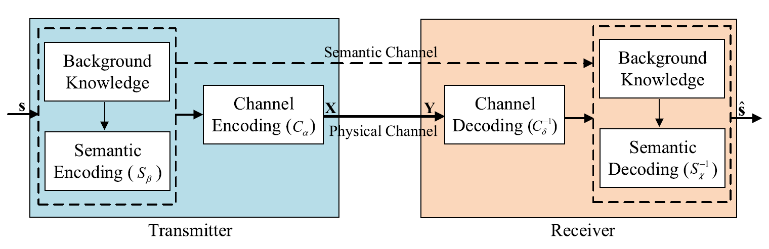
Semantic level에서는 semantic information을 추출하기 위한 encoding, decoding 즉, semantic information processing을 다룬다.

Transmission level에서는 semantic information이 transmission medium을 통해 정확히 교환될 수 있다는 것을 보장한다.

전반적으로 저자는 transmitter와 receiver가 특정 background knowledge를 갖는 즉, 다른 training data를 갖는 상황에서 stochastic (확률적인) physical channel을 고려하는 intelligent E2E 통신 시스템을 생각한다. 이때 background knowledge는 여러 application scenario에 따라 다양해질 수 있다.

Definition 1: Semantic noise는 message를 주고 받을 때, message transmission에 사용된 단어나 문장 혹은 symbol의 모호함 등으로 인해 message의 해석이 어려워지도록 하는 방해의 한 종류이다.
Definition 2: Physical channel noise는 physical channel impairment에 의해 발생한다. 예를 들면 signal attenuation과 distortion을 발생시키는 AWGN, fading channel, multiple path 등이 있다.

Problem Description

Fig. 1에서 볼 수 있듯이 transmitter는 문장 $\mathbf{s}$를 complex symbol stream $\mathbf{x}$로 mapping 하고, 이를 distortion과 noise가 있는 physical channel을 통해 전송한다. 수신된 $\mathbf{y}$는 receiver에서 original sentence $\mathbf{s}$를 추정하기 위해 decoding 된다. 저자는 transmitter와 receiver를 DNNs를 사용하여 동시에 설계한다. 왜냐하면 DL을 이용하면, 각자 길이가 다른 (variable-length) 문장과 다른 언어를 입력해도 model을 학습할 수 있기 때문이다.

다시 Fig. 1을 보자. Transmitter 는 semantic encoder와 channel encoder 두 부분으로 구성되는데, 이는 $\mathbf{s}$ 로부터 semantic information을 잘 얻어내어 physical channel을 통해 성공적인 전송을 하는 것을 보장하기 위함이다.

한편, DeepSC의 input을 문장 $\mathbf{s} = [w_1, w_2, \cdots, w_L]$ 로 두자. 이때 $w_l$은 문장에서의 $l$ 번째 단어를 의미한다. 그렇다면 encoding 된 symbol stream은 $\mathbf{x} = C_{\boldsymbol{\alpha}}(S_{\boldsymbol{\beta}}(\mathbf{s}))$ 로 표현할 수 있다. 이때 $\mathbf{x} \in \mathbb{C}^{M \times 1}$ 이고, $S_{\boldsymbol{\beta}}(\cdot)$는 parameter set $\boldsymbol{\beta}$를 이용한 semantic encoder network, $C_{\boldsymbol{\alpha}}(\cdot)$은 set $\boldsymbol{\alpha}$를 이용한 channel encoder를 의미한다.

쉬운 분석을 위해 coherent time을 $M$ 이라 가정하자. 만약 $\mathbf{x}$가 전송되었다면 receiver에 도착한 신호는 $\mathbf{y} = h\mathbf{x} + \mathbf{n}$ 이 될 것이다.
($\mathbf{y} \in \mathbb{C}^{M \times 1}$ 이고, $h$는 $\mathcal{C}N(0, 1)$의 Rayleigh fading channel, $\mathbf{n} \sim \mathcal{C}N(0, \sigma^2_n)$ 이다.)

Encoder와 decoder의 E2E 학습을 위해 channel은 back-propagation이 가능해야 한다. Physical channel은 neural networks (NNs)로 구성할 수 있다. 예를 들어 간단한 NNs를 사용하면 AWGN, multiplicative Gaussian noise, erasure channel 등을 modeling 할 수 있다. Fading channel의 경우 더 복잡한 network가 필요하지만, 본 논문에서는 AWGN과 Rayleigh fading channel만 간단히 고려하고 semantic coding 및 decoding에 더 집중한다.

Receiver 는 전송된 symbol을 복원하기 위한 channel decoder와 전송된 문장을 복원하기 위한 semantic decoder로 구성된다. 이때 decoded signal은 $\hat{\mathbf{s}} = S^{-1}_{\boldsymbol{\chi}}(C^{-1}_{\boldsymbol{\delta}}(\mathbf{y}))$ 와 같이 표현할 수 있다. 이전과 비슷하게 $\hat{\mathbf{s}}$ 는 복원된 문장을 의미하고, $C^{-1}_{\boldsymbol{\delta}}(\cdot)$는 parameter set $\boldsymbol{\delta}$를 이용한 channel decoder, $S^{-1}_{\boldsymbol{\chi}}(\cdot)$은 set $\boldsymbol{\chi}$를 이용한 semantic decoder를 의미한다.

이 system의 목표는 전송시키는 symbol의 개수를 줄이는 동시에 semantic error를 최소화 시키는 것이다. 하지만 여기서 우리는 두 가지 challenge에 직면하게 된다. 첫 번째는 joint semantic-channel coding을 어떻게 설계할 것인가 이고, 다른 하나는 semantic transmission (기존의 통신 시스템에서 고려된 적 없음) 이다. 비록 기존의 통신 시스템으로 낮은 BER을 얻을 수 있지만, noise 혹은 error correction 능력을 넘어선 상황으로 인해 왜곡된 여러 개의 bits는 전체 문장이 가지고 있던 semantic information 중 일부를 잃어 이해를 어렵게 만들 수 있다.

Semantic level에서의 성공적인 복원을 위해, 우리는 semantic coding과 channel coding을 동시에 설계하여 $\hat{\mathbf{s}}$ 과 $\mathbf{s}$ 사이 의미를 유지할 것이다. 이 둘의 차이를 계산하기 위해서는 cross-entropy (CE)가 loss 함수로 사용되는데 식은 다음과 같다.

여기서 $q(w_l)$은 estimated sentence $\mathbf{s}$에 $l$ 번째 단어 $w_l$이 등장할 real 확률을 의미하고, $p(w_i)$은 문장 $\hat{\mathbf{s}}$에 $i$ 번째 단어 $w_i$가 등장할 predicted 확률을 뜻한다.

CE는 두 확률 분포의 차이를 측정할 수 있다. 따라서 CE의 loss 값을 줄이면 network는 source sentence $\mathbf{s}$ 에서 단어의 분포 $q(w_l)$을 학습할 수 있다. 이말인즉슨 문맥상 구문, 관용구, 단어의 의미 등을 network로 학습할 수 있다는 것을 뜻한다.

게다가 semantic-channel coding을 동시에 설계하고 학습하면, 전체 network가 특정 목적을 위한 지식을 학습하도록 만들 수 있다. 다시 말하면 channel coding은 transmission 목적과 관련이 없는 정보들은 무시하면서, semantic information을 보호하는 것에 더 집중할 수 있다. 만약 둘을 따로 설계한다면, channel coding은 모든 정보들을 동일하게 다루도록 만들어질 것이다.

Channel Encoder And Decoder Design

Communication system을 설계하는 것에 있어서 중요한 목표 중 하나는 data 전송 rate 혹은 capacity를 최대화 하는 것이다. BER과 비교해봤을 때, mutual information은 receiver를 학습시키기 위한 추가 정보를 제공할 수 있다. 전송된 symbol $\mathbf{x}$와 수신 symbol $\mathbf{y}$의 mutual information은 다음과 같이 계산된다. ($p(x)$는 $\mathbf{x}$를 보내는 것에 대한, $p(y)$는 $\mathbf{y}$를 받는 것에 대한 marginal probability)

Mutual information은 marginal probabilities와 joint probability 사이의 Kullback-Leibler (KL) divergence와 같다.
$\rightarrow$ 즉, $I(\mathbf{x}; \mathbf{y}) = D_{\textrm{KL}}(p(x,y)||p(x)p(y))$

한편 다음의 theorem을 보자.

Theorem 1: KL divergence admits the following dual representation.
$D_{\textrm{KL}} (P||Q) = \sup\limits_{T: \Omega \rightarrow R} E_P[T] - \log (E_Q[e^T])$
(Supremum은 두 expectation이 finite 하도록 하는 모든 function $T$ 중에서 선택된다.)

Theorem 1에 의해 KL divergence는 다음과 같이 표현될 수 있다.

즉, $I(\mathbf{x}; \mathbf{y})$의 lower bound를 얻을 수 있다. 위의 식을 $(*)$ 라 두자.

$I(\mathbf{x}; \mathbf{y})$의 더 tight 한 bound를 찾기 위해서 unsupervised method를 사용하여 network $T$ 를 학습해보자. 한편 $(*)$ 의 기대값은 sampling을 통해 계산될 수 있다. (Sample 수가 증가할수록 true value로 수렴). 그렇다면 우리는 $(*)$ 에 정의된 mutual information을 최대화 하여 encoder를 최적화 할 수 있고, 관련된 loss function은 다음과 같이 주어진다.

논문의 proposed design에서 $\mathbf{x}$는 function $C_{\boldsymbol{\alpha}}$와 $S_{\boldsymbol{\beta}}$에 의해 생성되기 때문에 loss function은 $\mathcal{L}_{\textrm{MI}}(\mathbf{x}, \mathbf{y}; T,\boldsymbol{\alpha},\boldsymbol{\beta})$와 같이 표현되고, 다음의 관계식이 성립한다.

이때, $(**)$ 의 loss 함수는 $\boldsymbol{\alpha}$, $\boldsymbol{\beta}$, $T$ 를 얻기 위한 NNs의 학습을 위해 사용될 수 있다.

예를 들면 encoder $\boldsymbol{\alpha}$와 $\boldsymbol{\beta}$가 고정되었을 때, network $T$를 학습하여 mutual information을 추정할 수 있다. 이와 비슷하게 mutual information을 얻으면, $\boldsymbol{\alpha}$와 $\boldsymbol{\beta}$를 학습하여 encoder를 최적화 할 수 있다.

Performance Metrics

System design에 있어서 performance 측정 기준은 매우 중요하다. E2E communication system에서 training target으로 BER이 종종 사용되기도 하지만, 앞선 포스팅에서 언급했던 바와 같이 text transmission task에 대해 BER은 performance를 잘 반영할 수 없다. 따라서 본 논문에서 사용될 다음의 두 metric을 소개한다.

BLEU Score

Transmitted와 received texts 사이의 $n$-grams 차이를 세는 방법이다. 이때 $n$-grams 란 word group의 size를 의미한다.

예시) 문장: 'weather is good today'
1-gram: 'weather', 'is', 'good', 'today'.
2-grams: 'weather is', 'is good', 'good today'.

길이 $l_{\mathbf{s}}$의 transmitted sentence $\mathbf{s}$ 와 길이 $l_{\hat{\mathbf{s}}}$의 decoded sentence $\hat{\mathbf{s}}$ 에 대한 BLEU의 식은 아래와 같다.
($u_n$: weights of $n$-grams, $p_n$: $n$-grams score, $C_k(\cdot)$: $n$-grams의 $k$ 번째 elements에 대한 frequency count function)

BLEU의 output 범위는 0부터 1까지 이고, 이는 decoded text 가 원래의 text 와 얼마나 유사한지를 나타낸다.

하지만, word의 error가 항상 문장의 의미를 바꾼다고 말할 수는 없다. 즉, BLEU score는 semantic information을 비교한다기 보다 오직 두 문장의 단어 차이를 비교하기 때문에 저자는 sentence similarity라는 새로운 metric을 함께 제시한다.

Sentence Similarity

단어는 맥락마다 다른 의미를 가질 수 있다. (우리나라의 동음이의어를 생각하자). 따라서 저자는 semantic similarity에 따라 문장의 유사성을 계산하도록 다음의 방식을 제안한다.

이때 $\mathbf{s}$와 $\hat{\mathbf{s}}$는 각각 기존/복원된 문장을, $\mathbf{B}_{\boldsymbol{\Phi}}$는 pre-trained BERT 모델을 의미한다. 또한 위의 식은 decoded sentence 가 원래의 sentence 와 얼마나 유사한지를 나타낸다. (BLEU와 다른 부분)

정리하면 semantic information에 대해 학습한 BERT를 사용하여 문장 $\mathbf{s}$에 숨어있는 semantic information $\mathbf{c}$를 얻어내고, 이를 통해 sentence similarity를 계산할 수 있다.

Proposed Deep Semantic Communication Systems

Basic Model

제안한 DeepSC 모델은 아래의 Fig. 2와 같다.

Fig. 2. Semantic communication system을 위해 제안된 neural network 구조

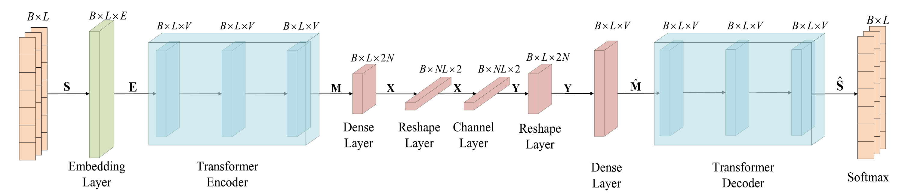
Transmitter 는 semantic encoder 와 channel encoder 로 이루어져 있는데, semantic encoder는 전송할 semantic feature를 text로부터 얻어 내기 위해 사용되고, channel encoder는 다음 전송을 가능하도록 하는 symbol을 생성한다.

이러한 semantic encoder는 여러 개의 transformer encoder layer로 구성되고, channel encoder는 다른 unit을 가지는 dense layer들을 통해 구현된다. 또한 AWGN channel은 model에서 하나의 layer로 표현된다.

마찬가지로 receiver 는 symbol detection을 위한 channel decoder 와 text의 추정을 위한 semantic decoder 로 구성되는데, channel decoder는 다른 unit을 가지는 dense layer들, semantic decoder는 여러 개의 transformer decoder layer로 표현된다.

Loss 함수의 구성은 다음과 같다.

Loss의 첫 번째 항은 sentence similarity에 대한 것으로, 전체 system의 학습을 통해 $\mathbf{s}$와 $\hat{\mathbf{s}}$의 semantic difference를 최소화하는 것이 목표이다.

두 번째 항은 mutual information을 위한 것으로, transmitter의 학습 과정에서 achieved data rate을 최대화한다. 참고로 $\lambda$는 두 번째 항을 위한 weight 이다.

Transformer의 핵심은 multi-head self-attention mechanism 이다. 이는 transformer로 하여금 sequence 안에서 이전에 예측했던 단어를 보게 해주어, 다음 단어의 예측을 더 잘 하도록 만들어준다. Transformer에 대한 자세한 내용은 2017년에 발표된 원 논문 "Attention is all you need." 를 참고하기로 하고 (code도 함께 보면 좋아 'paperswithcode' 링크를 첨부했습니다), 여기서의 핵심은 self-attention mechanism을 통해 semantic 정보를 학습할 수 있다는 것임을 기억하자.

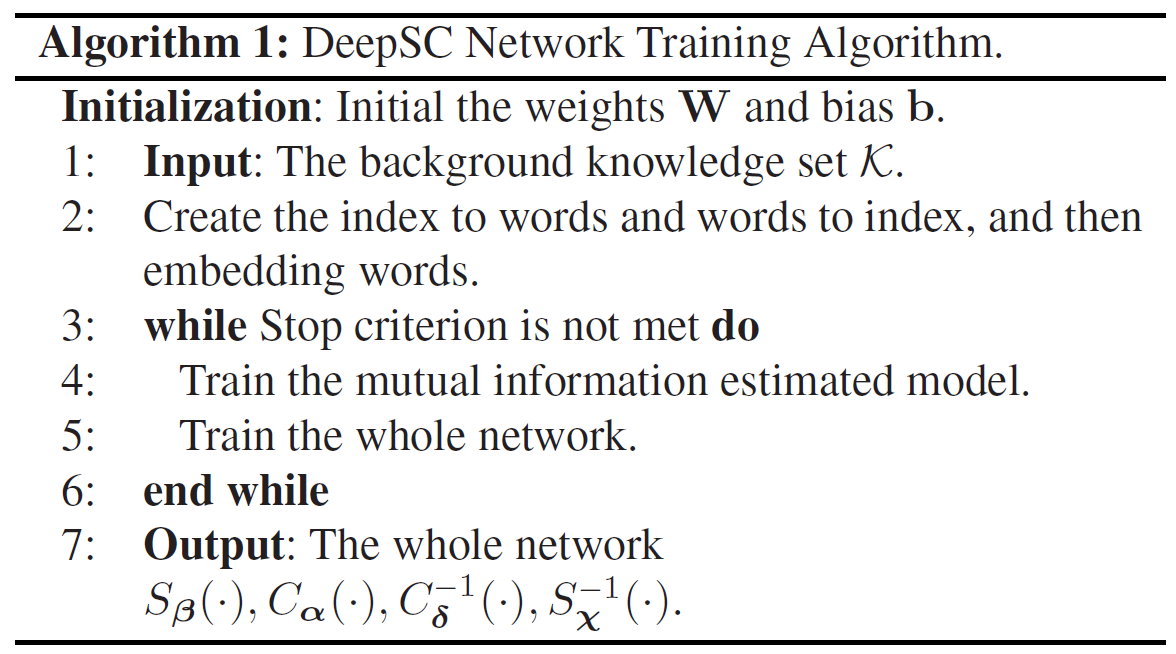
DeepSC의 training process는 서로 다른 loss function으로 인하여 두 개의 phase로 구분된다. 아래의 Algorithm 1을 보자.

Algorithm 1: DeepSC network training algorithm.

• Weight와 bias를 초기화 한 뒤, embedding vector를 이용하여 input word를 표현한다.
• 첫 번째 phase는 두 번째 phase를 위한 achieved data rate을 추정하기 위해 unsupervised learning으로 mutual information model을 학습하는 과정이다.
• 두 번째 phase는 $\mathcal{L}_\textrm{total}$ 을 loss function으로 설정하여, 전체 system을 학습하는 단계이다.
• 각 phase의 목표는 loss 함수를 최소화 하는 것이다. Stop 기준에 부합하거나 최대 iteration 횟수에 도달 혹은 loss function의 개선이 더 없으면 종료된다.
  

다시 강조하지만 기존의 방식대로 semantic coding과 channel coding을 따로 진행하면 encoder/decoder는 digital bits 만을 다루게 될 것이다. 하지만 joint semantic-channel coding을 사용하면 data를 압축할 때도 semantic information을 보존할 수 있다.

이제 두 training phase를 더 자세히 살펴보자.

Training of Mutual Information Estimation Model

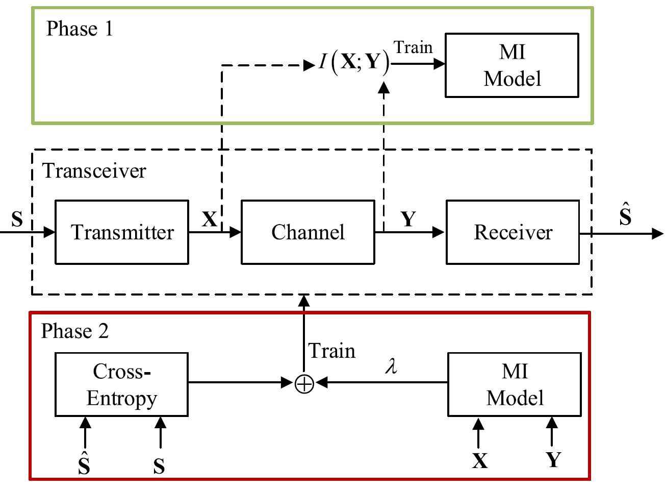
아래의 Fig.3 과 Algorithm 2는 mutual information 추정 모델의 학습 과정을 나타낸다.

Fig. 3. DeepSC의 training framework
Phase 1: Mutual information estimation model을 학습.
Phase 2: Cross-entropy와 mutual information을 기반으로 전체 network를 학습.

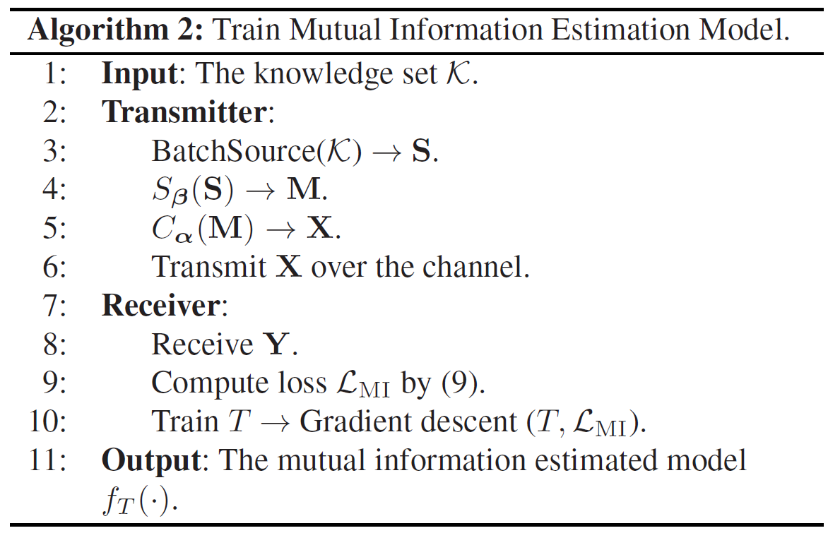
Algorithm 2: Train mutual information estimation model.

• 먼저 knowledge set $\mathcal{K}$는 문장들의 minibatch $\mathbf{S}\in \Re^{B\times L \times 1}$ 를 생성한다. ($B$는 batch size, $L$은 문장 길이를 의미)
• Embedding layer를 통해 문장은 dense word vector $\mathbf{E}\in \Re^{B\times L \times E}$로 표현될 수 있다. 이때 $E$는 word vector의 차원이다.
• Semantic encoder layer를 통과하여 $\mathbf{M}\in \Re^{B\times L \times V}$을 얻는다. 이때 $V$는 transformer encoder output의 차원이다.
• $\mathbf{M}$은 physical channel의 영향에 대처하기 위해 symbol $\mathbf{X} \in \Re^{B\times NL \times 2}$로 encoding 된다. Channel을 지나가면 receiver는 channel noise에 의해 왜곡된 신호 $\mathbf{Y}$를 얻는다.
• 송신 symbol $\mathbf{X}$와 수신 symbol $\mathbf{Y}$를 기반으로 loss $\mathcal{L}_{\textrm{MI}}$ 를 계산한다. 이후 SGD를 이용하여 $f_T(\cdot)$를 update 한다.
  

Whole Network Training

전체 network 학습 과정은 Algorithm 3과 같다.

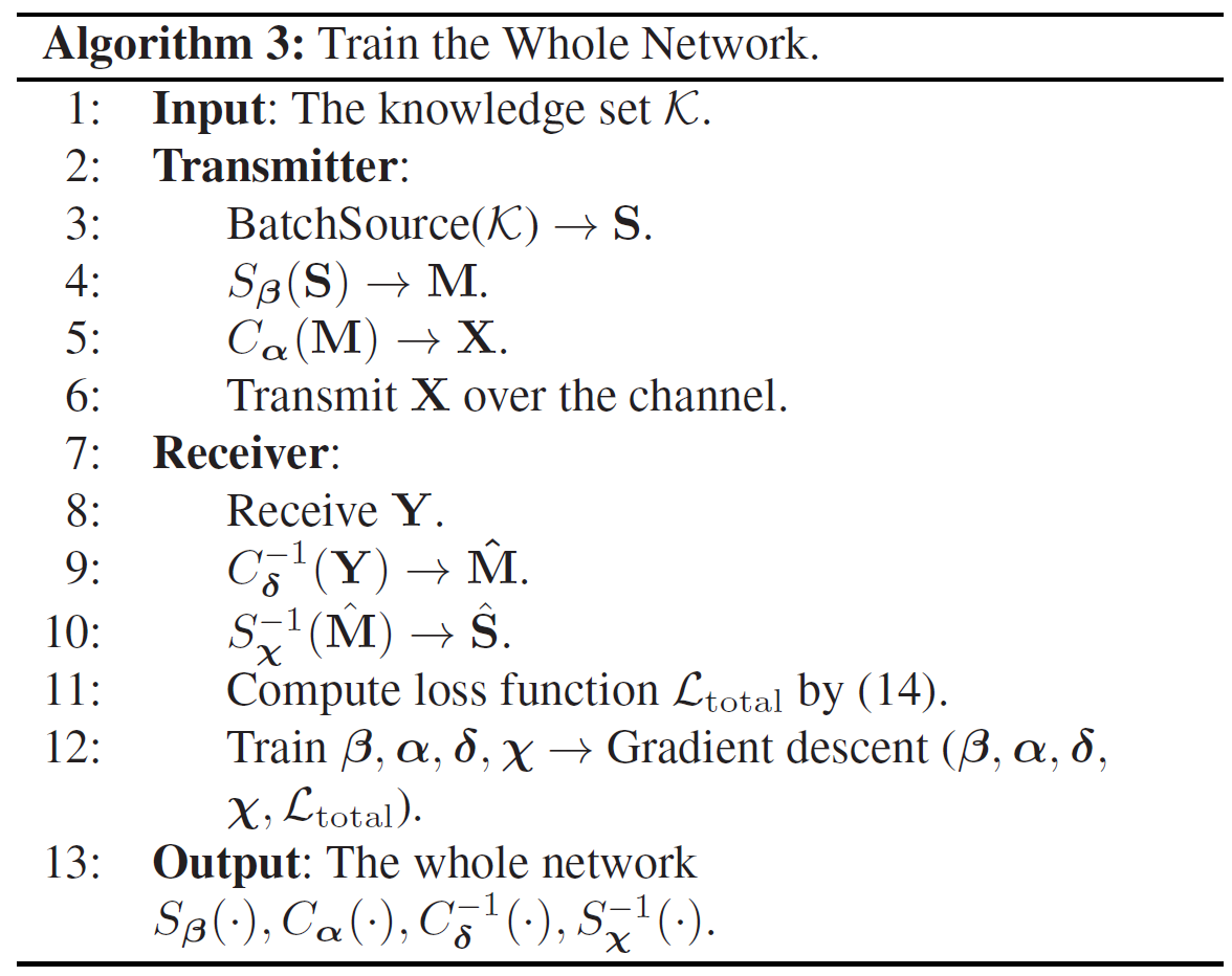
Algorithm 3: Train the whole network.

• Knowledge set $\mathcal{K}$ 에서 만들어진 minibatch $\mathbf{S}$가 semantic level에서 $\mathbf{M}$으로 encoding 된다.
• $\mathbf{M}$은 symbol $\mathbf{X}$로 encoding 되어 physical channel을 통해 전송된다.
• Receiver 단에서는 channel에 의해 왜곡된 $\mathbf{Y}$를 받고, channel decoder layer를 통해 decoding 한다. 이때 $\hat{\mathbf{M}}\in \Re^{B\times L \times V}$은 복원된 source의 semantic information 이다.
• 전송된 문장은 semantic decoder layer를 통해 추정된다.
• $\mathcal{L}_{\textrm{total}}$ 을 기반으로 SGD를 수행하여 network를 학습한다.
  

Transfer Learning For Dynamic Environment

실제 상황을 생각해보면, 다른 통신 scenario는 곧 다른 channel과 training data를 가지고 있다는 것을 의미한다. 이때 re-training을 빨리 진행시키기 위한 deep transfer learning 방식을 알아보자.

Fig. 4와 Algorithm 4는 transfer learning을 위한 training 과정을 설명하고 있는데, 이때 training modules와 앞서 설명한 두 가지 training 방식은 Algorithm 2, 3과 같다.

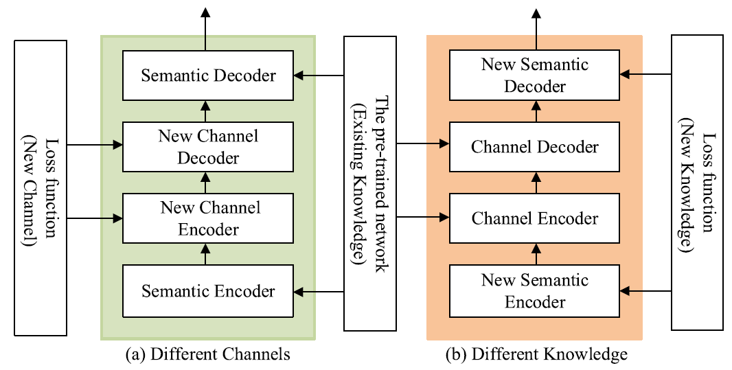
Fig. 4. Transfer learning based training framework
(a): 다른 channel에 대해 channel encoder/decoder 재학습
(b): 다른 background knowledge에 대해 semantic encoder/decoder 재학습

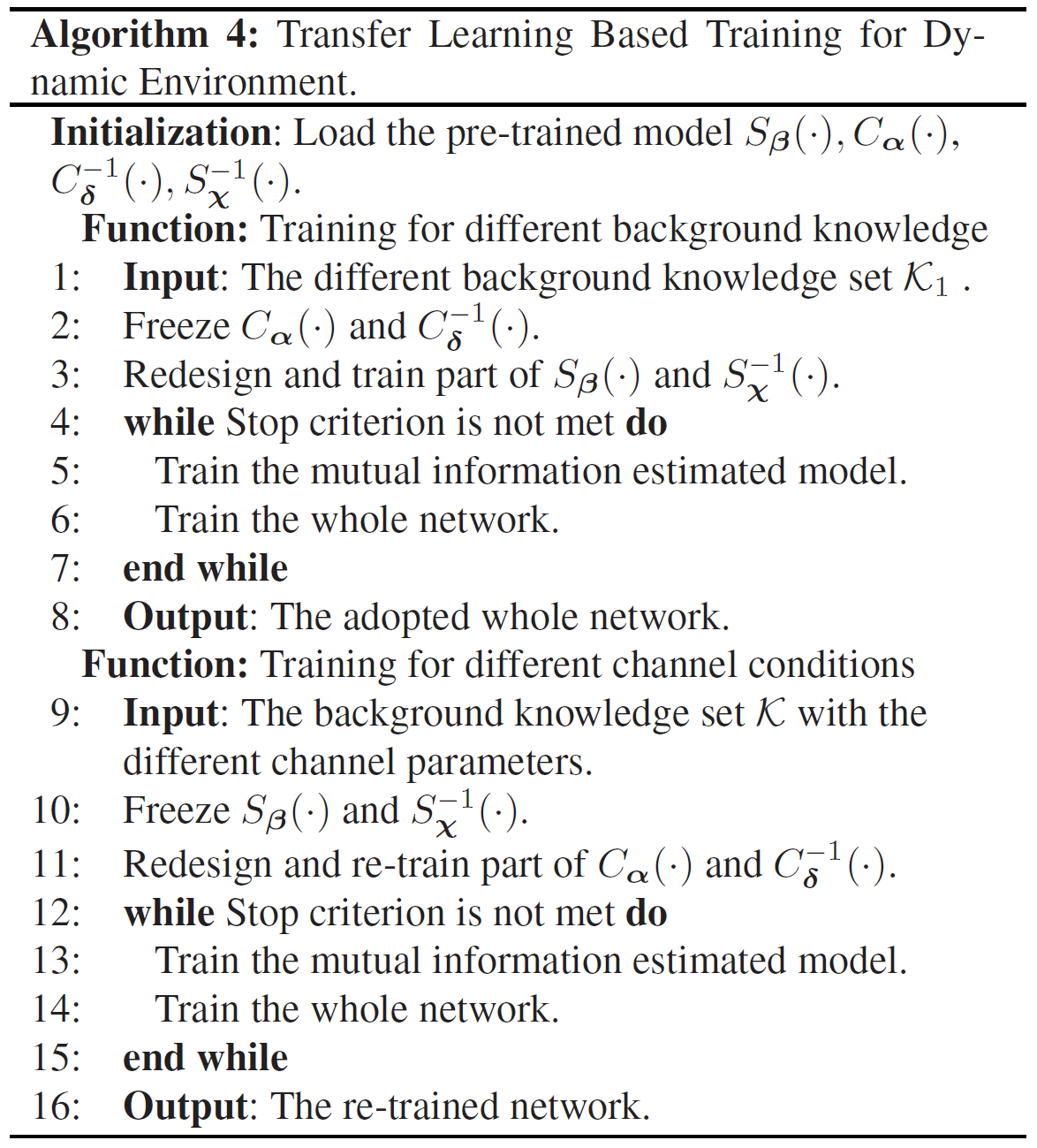
Algorithm 4: Transfer learning based training for dynamic environment.

• Knowledge $\mathcal{K}_0$ 와 channel $\mathcal{N}_0$ 에서 미리 학습된 transmitter와 receiver를 load 한다.
• Case 1) Background knowledge가 달라진 경우
  $\Rightarrow$ Freeze channel encoder/decoder, re-train semantic encoder/decoder.
• Case 2) Communication 환경이 달라진 경우
  $\Rightarrow$ Freeze semantic encoder/decoder, re-train channel encoder/decoder.
• Case 3) 둘 다 달라진 경우
  $\Rightarrow$ Re-train 진행. 하지만 이 경우에도 pre-trained transceiver는 학습에 필요한 시간을 줄일 수 있다.
  

Reference

Xie, Huiqiang, et al. "Deep learning enabled semantic communication systems." IEEE Transactions on Signal Processing 69 (2021): 2663-2675.

DeepSC - PyTorch Official code.