논문 및 이미지 출처 : https://ojs.aaai.org/index.php/AAAI/article/view/19885
Abstract
- Handwritten Mathematical expression Recognition (HMER) 는 이미지로 LaTeX 생성이 목적이며, 최근 attention 기반의 encoder-decoder 모델이 널리 사용.
- 일반적으로 left-to-right (L2R) sequence 이며, R2L 은 활용되지 않음
- 본 논문은 Attention Aggregation based Bi-direction Mutual Learning Network (ABM) 제안
- 하나의 encoder 를 공유하고 역방향 병렬 decoder (L2R, R2L) 두 개를 구성
- 두 decoder 는 상호간섭으로 성능향상
- 다양한 수학 기호 처리를 위해 Attention Aggregation Module (AAM) 제안
- 다중 스케일 어텐션을 효과적으로 통합
- 추론 단계에서, L2R branch 만 사용하여 기존 매개변수 및 추론 속도 유지
code - https://github.com/WH-B/ABM
Introduction
보통 LaTeX sequence 생성법은 설계된 문법에 의존한다.
이 문법은 수학식 구조, 기호 위치 관계 및 파싱 알고리즘을 정의하기 위해서는 광범위한 사전 지식이 필요하다.
최근 HMER 에 어텐션을 적용하여 우수한 성능을 보인다.
- WAP : coverage 부족 문제 해결을 위해 2D coverage attention 도입
- past attention 의 합으로, historical align 정보를 추적하여 높은 확률을 할당하도록 가이드
- historical align 정보만 사용하여 future 정보는 고려하지 않음 (attention drift problem)
예; "{" 과 "}" 는 항상 함께 나타나며 떨어져있음
- BTTR : attention drift 해결을 위해 두 가지 방향을 갖는 transformer decoder 사용
- 반대 방향에서 학습할 명시적 정보가 없으며 coverage 매커니즘 없이 attention 을 align
- 위 문제로 장문의 수식이나 다양한 크기의 수식에 일부 제한이 있음
- DWAP-MSA : 위 문제 해결을 위해 다중 스케일 피쳐를 인코딩 시도
- 로컬 수용 영역은 조절하지 않고 피쳐 맵만 조정하여 작은 문자를 정확히 인식하기 어려움
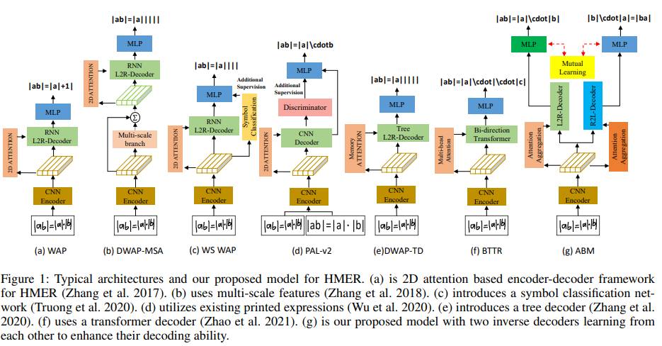
- ABM : 세 개의 모듈 포함
- Feature Extraction module (FEM)
WAP 에서 효과를 증명한 DenseNet 사용 - Attention Aggregation Module (AAM)
multi-scale coverage attention 으로 다양한 크기의 수식 인식 정확도를 향상시키고 오류 완화 - Bi-directional Mutual Learning Module (BMLM)
두 병렬 디코더로 새로운 디코더 프레임워크를 제안하며 상호 지식 전달로 서로 학습
coverage attetion 의 historical 과 future 를 충분히 활용하여 위치 결정
추론 시에는 L2R branch 만 사용
- Feature Extraction module (FEM)
contribution 을 세 가지로 요약한다.
- 공유되는 encoder 와 두 역방향 decoder 로 새로운 bi-directional mutual learning 제안.
- multi-scale coverage attention 매커니즘으로 다양한 크기 인식
- ABM 은 GRU, LSTM, Transformer 를 포함한 다양한 decoder 를 적용 가능
Related Work
Method
Feature Extraction Module
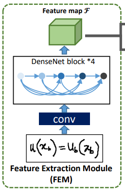
WAP 과 유사하게, DenseNet 을 encoder 로 사용하여 이미지의 특징을 추출한다.
이 출력은 인 3차원 피처맵 이다.
저자는 output feature 를 차원의 content information a 로 간주한다.
여기서 vector a = 이며 , 이다.
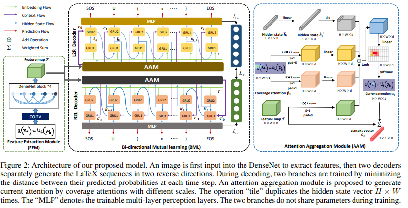
Attention Aggregation Module
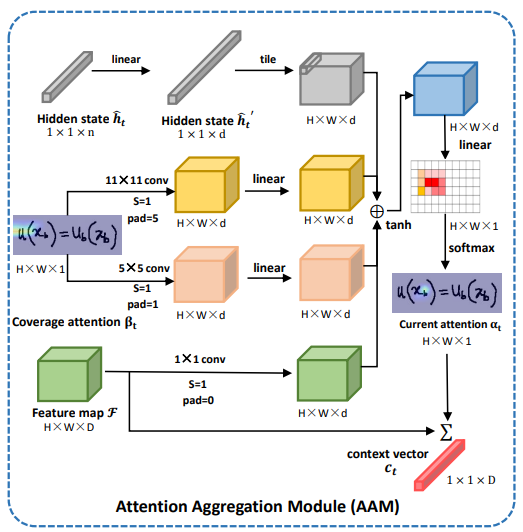
coverage 기반 attention 은 align information 을 잘 추적하고, 번역되지 않은 영역에 높은 확률로 가이드한다.
Inception Module 에 영감을 받아 AAM 을 제안하여 coverage attention 에서 다양한 수용 영역을 집계한다.
AAM 은 로컬 영역의 상세한 특징과 더 큰 수용 영역으로 전역 정보에도 주목할 수 있다.
DWAP-MSA 는 다중 스케일 브랜치를 밀집 인코더로 제안한 다른 개념이며 저/고해상도 특성을 생성하지만 많은 매개 변수와 계산을 필요로 한다.
hidden state , feature map 그리고 coverage attetion 를 사용하여 current attention weight 를 계산한 후 context vector 를 얻는다.
와 은 크고 작은 커널 사이즈 (예5, 11)의 convolution 작업을 나타낸다.
는 모든 past attention 확률의 합을 나타내며, 0 vector 로 초기화된 후 다음으로 계산 된다.
여기서 는 step 의 attention score 를 나타낸다.
current attention map 는 다음과 같이 계산된다.
여기서 , 그리고 은 학습 가능한 weight matrices 이다.
는 1x1 convolution 이며 는 GRU 로 생성된 hidden state 이다.
context vector 는 로 나타내며, content information a 피처의 weighted sum 으로 계산된다.
여기서 는 step 에서의 의 -th 피처의 weight 이다.
Bi-directional Mutual Learning Module

일반적으로 long-distance dependence 를 고려하지 않은 L2R 방법을 사용한다. 그래서 두 방향 (L2R, R2L) 으로 LaTeX sequence 를 생성하는 dual-stream decoder 를 제안한다.
두 branch 는 같은 아키텍처이지만, 디코딩 방향이 다르다.
bi-directional training 의 경우, 와 를 LaTeX sequence 의 시작과 끝으로 추가한다.
target LaTeX sequence 의 길이 , 일 경우
- L2R :
- R2L :
L2R 과 R2L branch 에 대한 step t 에서의 예측되는 symbol 의 확률은 다음과 같이 계산한다.
여기서 , 는 L2R branch 의 step 에서의 현재 상태와 이전 예측 아웃풋이다.
마커는 R2L branch 를 나타낸다.
- , , 그리고 는 훈련 가능한 행렬
- , , 은 attention 차원, symbol class 의 수, GRU 차원
- 는 임베딩 행렬
- 는 maxout activation function
hidden representation 은 다음과 같이 생성된다.
- 와 는 WAP 과 유사한 unidirectional GRU 모델이다.
L2R branch 의 확률을
R2L branch 는 으로 나타낸다.
여기서 는 -th step 디코딩 수형할 때의 label symbols 의 예측되는 확률이다.
두 branch 로부터의 예측 분포에 mutual learning 을 적용하기 위해, L2R 및 R2L decoder 로 생성된 LaTeX sequence 를 align 할 필요가 있다.
및 을 얻기 위해 첫 번째와 마지막 예측 ( 및 ) 을 버린다.
그리고 을 얻기 위해서는 를 역전시킨다.
동시에, 이 둘 사이의 확률 분포의 다양하게 수량화하기 위해 Kullback-Leibler (KL) Loss 를 사용한다.
훈련 중, 더 많은 정보 제공을 위해 모델로 생성된 soft probabilities 를 사용한다. 따라서, L2R branch 로부터의 soft probability categories 는 다음과 같이 정의된다.
- 는 soft labbel 생성에 대한 temperature parameter
- 이 sequence 의 -th symbol 의 logit 은 로 정의된 decoder network 로 계산
목표는 두 branch 의 확률 분포간의 거리를 최소화하는 것이므로, 및 간의 KL distance 는 다음과 같이 계산된다.
- 는 다른 branch 에서의 ground-truth 와 확률 분포로 모델 훈련에 경쟁력있는 contribution 을 만들어준다.
- 및 은 L2R 과 R2L 의 logit 을 나타낸다.
Loss Function
target LaTeX sequence 의 길이 , 의 경우, -th time step 에서 가 있는 로 해당하는 one-hot grount-truth 을 나타낸다.
-th symbol 의 softmax 확률은 다음과 같이 계산한다.
multi-class classification 의 경우, 두 branch 에 대한 target label 과 softmax 확률 간의 cross-entropy loss 는 다음과 같이 정의된다.
전체 loss function 은 다음과 같이 계산한다.
여기서 는 recognition loss 와 KL divergence loss 의 밸런스를 위한 hyper-parameter 이다.
Experiment
Datasets and Metrics
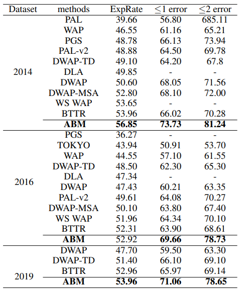
CROHME 2014, 2016, 2019 데이터셋으로 평가를 진행한다.
두 가지 지표로 ExpRate(%) <= 1 error (%) <= 2 error (%) 로 구조적 또는 기호 오류가 허용되는 경우의 표현식 인식 정확도를 나타낸다. 다른 한 가지는 단어 오류율 (WER(%)) 로, 단어 수준에서 대체, 삭제 및 삽입과 같은 오류를 평가하는데 사용된다.
Implementation Details
Setup
두 가지의 다른 decoder branch 는 서로 다른 초기화 방법을 사용한다.
decoder 의 경우, n=256, d=512, D=684 및 K=113 으로 설정하며 는 0.5 로 설정된다.
Training
Adadelta 옵티마이저로 최적화하며 학습률은 1 에서 시작하여 WER 이 15 epoch 동안 감소하지 않을 때마다 두 배로 작아진다.
학습률이 10배로 감소할 때 훈련이 조기 종료된다.
배치 크기는 16으로 설정되었으며 모든 모델은 단일 NVIDIA V100 16GM GPU 에서 훈련/테스트 된다.