파이토치 기초 - 텐서 조작하기

벡터, 행렬 그리고 텐서(Vector, Matrix and Tensor)

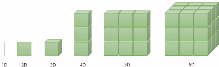
스칼라: 차원이 없는 값(위의 그림에는 없음),
벡터: 1차원으로 구성된 값
행렬(Matrix): 2차원으로 구성된 값
텐서(Tensor): 3차원으로 구성된 값

넘파이로 텐서 만들기(벡터와 행렬 만들기)

t = np.array([0., 1., 2., 3., 4., 5., 6.])
# 파이썬으로 설명하면 List를 생성해서 np.array로 1차원 array로 변환함.
print(t) #[0. 1. 2. 3. 4. 5. 6.]

print('Rank of t: ', t.ndim)
print('Shape of t: ', t.shape)

Rank of t:  1
Shape of t:  (7,)

벡터이므로 1차원이 출력된다.
(7, )는 (1, 7)을 의미한다.

t = np.array([[1., 2., 3.], [4., 5., 6.], [7., 8., 9.], [10., 11., 12.]])
print(t)

[[ 1.  2.  3.]
 [ 4.  5.  6.]
 [ 7.  8.  9.]
 [10. 11. 12.]]

print('Rank  of t: ', t.ndim)
print('Shape of t: ', t.shape)

Rank  of t:  2
Shape of t:  (4, 3)

이 때는 4행 3열인 2차원 행렬이 출력된다.

이제 넘파이가 아닌 파이토치로 텐서를 선언해보자.

t = torch.FloatTensor([0., 1., 2., 3., 4., 5., 6.])
print(t)

print(t.dim())  # rank. 즉, 차원
print(t.shape)  # shape
print(t.size()) # shape

1
torch.Size([7])
torch.Size([7])

1차원 텐서이고 원소는 7개이다.

인덱싱과 슬라이싱을 해보자.

print(t[0], t[1], t[-1])  # 인덱스로 접근
print(t[2:5], t[4:-1])    # 슬라이싱
print(t[:2], t[3:])       # 슬라이싱

tensor(0.) tensor(1.) tensor(6.)
tensor([2., 3., 4.]) tensor([4., 5.])
tensor([0., 1.]) tensor([3., 4., 5., 6.])

t = torch.FloatTensor([[1., 2., 3.],
                       [4., 5., 6.],
                       [7., 8., 9.],
                       [10., 11., 12.]
                      ])
print(t)

tensor([[ 1.,  2.,  3.],
        [ 4.,  5.,  6.],
        [ 7.,  8.,  9.],
        [10., 11., 12.]])

이 때는 (4,3)의 크기를 가진 2차원 텐서가 출력된다.

print(t[:, 1]) # 첫번째 차원을 전체 선택한 상황에서 두번째 차원의 첫번째 것만 가져온다.
print(t[:, 1].size()) # ↑ 위의 경우의 크기

tensor([ 2.,  5.,  8., 11.])
torch.Size([4])

print(t[:, :-1]) # 첫번째 차원을 전체 선택한 상황에서 두번째 차원에서는 맨 마지막에서 첫번째를 제외하고 다 가져온다.

tensor([[ 1.,  2.],
        [ 4.,  5.],
        [ 7.,  8.],
        [10., 11.]])

브로드캐스팅(Broadcasting)

• 불가피하게 크기가 다른 행렬 또는 텐서에 대해서 사칙 연산을 수행할 때 자동으로 크기를 맞춰 연산을 수행하는 것

m1 = torch.FloatTensor([[3, 3]])
m2 = torch.FloatTensor([[2, 2]])
print(m1 + m2)

tensor([[5., 5.]])

모두 둘 다 (1, 2)일 때는 문제 없이 연산이 되지만

# Vector + scalar
m1 = torch.FloatTensor([[1, 2]])
m2 = torch.FloatTensor([3]) # [3] -> [3, 3]
print(m1 + m2)

tensor([[4., 5.]])

m1의 크기는 (1, 2)
m2의 크기는 (1,)이다.
이 때 파이토치는 m2의 크기를 (1, 2)로 변경하여 연산을 수행한다.

# 2 x 1 Vector + 1 x 2 Vector
m1 = torch.FloatTensor([[1, 2]])
m2 = torch.FloatTensor([[3], [4]])
print(m1 + m2)

tensor([4., 5.],
       [5., 6.]])

m1의 크기는 (1, 2) m2의 크기는 (2, 1)이다.
이 때 파이토치는 두 벡터의 크기를 (2, 2)로 변경하여 덧셈을 수행한다.

# 브로드캐스팅 과정에서 실제로 두 텐서가 어떻게 변경되는지 보겠습니다.
[1, 2]
==> [[1, 2],
     [1, 2]]
[3]
[4]
==> [[3, 3],
     [4, 4]]

자주 사용되는 기능들

행렬 곱셈과 곱셈의 차이(Matrix Multiplication Vs. Multiplication)

m1 = torch.FloatTensor([[1, 2], [3, 4]])
m2 = torch.FloatTensor([[1], [2]])
print('Shape of Matrix 1: ', m1.shape) # 2 x 2
print('Shape of Matrix 2: ', m2.shape) # 2 x 1
print(m1.matmul(m2)) # 2 x 1

Shape of Matrix 1:  torch.Size([2, 2])
Shape of Matrix 2:  torch.Size([2, 1])
tensor([[ 5.],
        [11.]])

matmul을 사용해 2 x 2 행렬과 2 x 1 행렬(벡터)의 행렬 곱셈을 했다.

• 또는 mul()을 이용해 동일한 크기의 행렬이 동일한 위치에 있는 원소끼리 곱하는 연산을 해보자.

m1 = torch.FloatTensor([[1, 2], [3, 4]])
m2 = torch.FloatTensor([[1], [2]])
print('Shape of Matrix 1: ', m1.shape) # 2 x 2
print('Shape of Matrix 2: ', m2.shape) # 2 x 1
print(m1 * m2) # 2 x 2
print(m1.mul(m2))

Shape of Matrix 1:  torch.Size([2, 2])
Shape of Matrix 2:  torch.Size([2, 1])
tensor([[1., 2.],
        [6., 8.]])
tensor([[1., 2.],
        [6., 8.]])

m1 행렬의 크기는 (2, 2) m2 행렬의 크기는 (2, 1)이었다.
이때 element-wise 곱셈을 수행하면, 두 행렬의 크기는 브로드캐스팅이 된 후에 곱셈이 수행된다.

# 브로드캐스팅 과정에서 m2 텐서가 어떻게 변경되는지 보겠습니다.
[1]
[2]
==> [[1, 1],
     [2, 2]]

평균

t = torch.FloatTensor([1, 2])
print(t.mean())

tensor(1.5000)

t = torch.FloatTensor([[1, 2], [3, 4]])
print(t)

tensor([[1., 2.],
        [3., 4.]])

print(t.mean())

tensor(2.5000)

print(t.mean(dim=0))

tensor([2., 3.])

dim=0이라는 것은 첫번째 차원이고, 행렬에서 첫번째 차원은 행이다.
그리고 인자로 dim을 준다면 해당 차원을 제거한다는 의미가 됩니다. 즉 행렬에서 열만 남기겠다는 뜻이다.

기존 행렬의 크기는 (2, 2)였지만 이를 수행하면 열의 차원만 보존되면서 (1, 2), 즉 (2,)인 벡터이다.

# 실제 연산 과정
t.mean(dim=0)은 입력에서 첫번째 차원을 제거한다.

[[1., 2.],
 [3., 4.]]

1과 3의 평균을 구하고, 2와 4의 평균을 구한다.
결과 ==> [2., 3.]

인자로 dim=1을 주면 두번째 차원을 제거하여 열이 제거된 텐서가 된다.

print(t.mean(dim=1))

tensor([1.5000, 3.5000])

(2, 2)의 크기에서 (2, 1)의 크기가 된다.

# 실제 연산 결과는 (2 × 1)
[1. 5]
[3. 5]

dim=-1를 주는 경우 마지막 차원을 제거한다는 의미이고, 결국 열의 차원을 제거한다는 뜻이다.

print(t.mean(dim=-1))

tensor([1.5000, 3.5000])

덧셈

t = torch.FloatTensor([[1, 2], [3, 4]])
print(t)

tensor([[1., 2.],
        [3., 4.]])

print(t.sum()) # 단순히 원소 전체의 덧셈을 수행
print(t.sum(dim=0)) # 행을 제거
print(t.sum(dim=1)) # 열을 제거
print(t.sum(dim=-1)) # 열을 제거

tensor(10.)
tensor([4., 6.])
tensor([3., 7.])
tensor([3., 7.])

최대와 아그맥스

최대(Max)는 원소의 최대값을 리턴하고,
아그맥스(ArgMax)는 최대값을 가진 인덱스를 리턴한다

t = torch.FloatTensor([[1, 2], [3, 4]])
print(t)

print(t.max()) # Returns one value: max

tensor(4.)

print(t.max(dim=0)) # Returns two values: max and argmax

(tensor([3., 4.]), tensor([1, 1]))

행의 차원을 제거한다는 의미이므로 (1, 2) 텐서가 된다. 그런데 max에 dim 인자를 주면 argmax도 함께 리턴하게 된다.

# [1, 1]가 무슨 의미인지 봅시다. 기존 행렬을 다시 상기해봅시다.
[[1, 2],
 [3, 4]]
첫번째 열에서 0번 인덱스는 1, 1번 인덱스는 3입니다.
두번째 열에서 0번 인덱스는 2, 1번 인덱스는 4입니다.
다시 말해 3과 4의 인덱스는 [1, 1]입니다.

max 또는 argmax만 리턴받고 싶다면 다음과 같이 리턴값에도 인덱스를 부여한다.

print('Max: ', t.max(dim=0)[0])
print('Argmax: ', t.max(dim=0)[1])

Max:  tensor([3., 4.])
Argmax:  tensor([1, 1])

print(t.max(dim=1))
print(t.max(dim=-1))

(tensor([2., 4.]), tensor([1, 1]))
(tensor([2., 4.]), tensor([1, 1]))

뷰(View)

파이토치 텐서의 뷰(View)는 넘파이에서의 리쉐이프(Reshape)와 같은 역할이다.

t = np.array([[[0, 1, 2],
               [3, 4, 5]],
              [[6, 7, 8],
               [9, 10, 11]]])
ft = torch.FloatTensor(t)

print(ft.shape)

torch.Size([2, 2, 3])

print(ft.view([-1, 3])) # ft라는 텐서를 (?, 3)의 크기로 변경
print(ft.view([-1, 3]).shape)

tensor([[ 0.,  1.,  2.],
        [ 3.,  4.,  5.],
        [ 6.,  7.,  8.],
        [ 9., 10., 11.]])
torch.Size([4, 3])

print(ft.view([-1, 1, 3]))
print(ft.view([-1, 1, 3]).shape)

tensor([[[ 0.,  1.,  2.]],

        [[ 3.,  4.,  5.]],

        [[ 6.,  7.,  8.]],

        [[ 9., 10., 11.]]])
torch.Size([4, 1, 3])

스퀴즈(Squeeze)

차원이 1인 경우에는 해당 차원을 제거

ft = torch.FloatTensor([[0], [1], [2]])
print(ft)
print(ft.shape)

tensor([[0.],
        [1.],
        [2.]])
torch.Size([3, 1])

print(ft.squeeze())
print(ft.squeeze().shape)

(3 × 1)의 크기를 가지므로 squeeze를 사용하면 (3,)의 크기를 가지는 텐서로 변경된다.

언스퀴즈(Unsqueeze)

특정 위치에 1인 차원을 추가한다.

ft = torch.Tensor([0, 1, 2])
print(ft.shape)

torch.Size([3])

print(ft.unsqueeze(0)) # 인덱스가 0부터 시작하므로 0은 첫번째 차원을 의미한다.
print(ft.unsqueeze(0).shape)

tensor([[0., 1., 2.]])
torch.Size([1, 3])

(3,)의 크기를 가졌던 1차원 벡터가 (1, 3)의 2차원 텐서로 변경되었다. 그런데 이는 view로도 구현 가능하다.

print(ft.view(1, -1))
print(ft.view(1, -1).shape)

tensor([[0., 1., 2.]])
torch.Size([1, 3])

이번에는 unsqueeze의 인자로 1을 넣어보자.
두번째 차원에 1을 추가하겠다는 뜻이다.

print(ft.unsqueeze(1))
print(ft.unsqueeze(1).shape)

tensor([[0.],
        [1.],
        [2.]])
torch.Size([3, 1])

-1을 넣으면 어떻게 될까?
-1은 인덱스 상으로 마지막 차원을 의미하므로 마지막 차원에 1인 차원을 추가하면 (3, 1)의 크기가 된다.

print(ft.unsqueeze(-1))
print(ft.unsqueeze(-1).shape)

tensor([[0.],
        [1.],
        [2.]])
torch.Size([3, 1])

타입 캐스팅(Type Casting)

텐서의 각 자료형을 변환하는 것

lt = torch.LongTensor([1, 2, 3, 4])
print(lt)

이 long타입의 텐서를 float형으로 바꿔보자.

print(lt.float()) #tensor([1., 2., 3., 4.])

Byte 타입의 텐서를 만들어보자.

bt = torch.ByteTensor([True, False, False, True])
print(bt) #tensor([1, 0, 0, 1], dtype=torch.uint8)

이 바이트타입에 .long()이라고하면 long 타입의 텐서로 변경되고
.float()이라고 하면 float 타입의 텐서로 변경된다

print(bt.long())
print(bt.float())

tensor([1, 0, 0, 1])
tensor([1., 0., 0., 1.])

연결하기(concatenate)

x = torch.FloatTensor([[1, 2], [3, 4]])
y = torch.FloatTensor([[5, 6], [7, 8]])

이 두 텐서를 torch.cat을 사용해서 연결해보자.
torch.cat은 어느 차원을 늘릴 것인지를 인자를 줄 수 있다.

print(torch.cat([x, y], dim=0))

tensor([[1., 2.],
        [3., 4.],
        [5., 6.],
        [7., 8.]])

dim=0을 인자로 했더니 두 개의 (2 × 2) 텐서가 (4 × 2) 텐서가 되었다.

이번에는 dim=1을 해보자.

print(torch.cat([x, y], dim=1))

tensor([[1., 2., 5., 6.],
        [3., 4., 7., 8.]])

스택킹(Stacking)

연결을 하는 또 다른 방법이다.

x = torch.FloatTensor([1, 4])
y = torch.FloatTensor([2, 5])
z = torch.FloatTensor([3, 6])

torch.stack을 통해서 3개의 벡터를 모두 스택킹해보자.

print(torch.stack([x, y, z]))

tensor([[1., 4.],
        [2., 5.],
        [3., 6.]])

이 스태킹은 아래의 코드와 동일한 작업이다.

print(torch.cat([x.unsqueeze(0), y.unsqueeze(0), z.unsqueeze(0)], dim=0))

(2,)크기의 텐서 3개를 .unsqueeze(0)을 통해 (1, 2)의 크기의 2차원 텐서로 변경시키고
여기에 연결해서 사용하면 (3 x 2) 텐서로 만들었다.

또 스택킹에 dim 인자를 줄 수 있다.

print(torch.stack([x, y, z], dim=1))

tensor([[1., 2., 3.],
        [4., 5., 6.]])

dim=1을 통해 첫번째 차원이 증가하도록 쌓았고 결과적으로 (2 × 3) 텐서가 되었다.

ones_like, zeros_like

x = torch.FloatTensor([[0, 1, 2], [2, 1, 0]])
print(x)

tensor([[0., 1., 2.],
        [2., 1., 0.]])

이렇게 (2 × 3) 텐서를 만들었다. 이 텐서에 ones_like를 하면

print(torch.ones_like(x)) # 입력 텐서와 크기를 동일하게 하면서 값을 1로 채우기

tensor([[1., 1., 1.],
        [1., 1., 1.]])

1로 채워진 동일한 크기의 텐서가 만들어진다.

print(torch.zeros_like(x)) # 입력 텐서와 크기를 동일하게 하면서 값을 0으로 채우기

tensor([[0., 0., 0.],
        [0., 0., 0.]])

zeros_like는 동일한 크기의 0로 채워진 텐서가 만들어진다.

In-place Operation (덮어쓰기 연산)

x = torch.FloatTensor([[1, 2], [3, 4]])

print(x.mul(2.)) # 곱하기 2를 수행한 결과를 출력
print(x) # 기존의 값 출력

tensor([[2., 4.],
        [6., 8.]])
tensor([[1., 2.],
        [3., 4.]])

이 때 첫번째에 곱하기 2를 수행했지만
이를 x에다가 다시 저장하지 않았으니,
곱하기 연산을 하더라도 기존의 값 x는 변하지 않았다.

그런데 연산 뒤에 _를 붙이면 기존의 값을 덮어쓰기할 수 있다.

print(x.mul_(2.))  # 곱하기 2를 수행한 결과를 변수 x에 값을 저장하면서 결과를 출력
print(x) # 기존의 값 출력

tensor([[2., 4.],
        [6., 8.]])
tensor([[2., 4.],
        [6., 8.]])