14. Traditional Generative Models for Graphs
작성자: 14기 김상현
Graph Generation
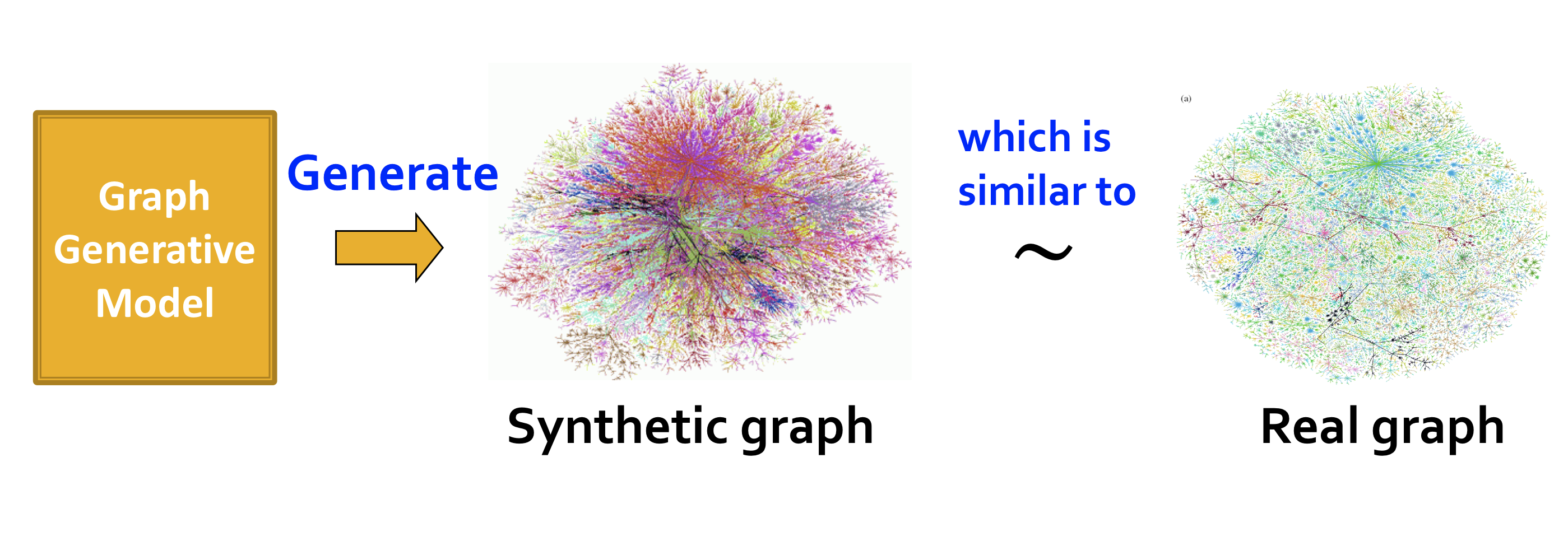
그래프 생성 모델(Graph Generative Model)을 통해 실제 그래프와 유사한 그래프를 생성한다.
그래프 생성을 공부하는 이유는 다음과 같다.
- Insights
- Predictions
- Simulations
- Anomaly detection
Properties of Real-world Graphs
Network Properties
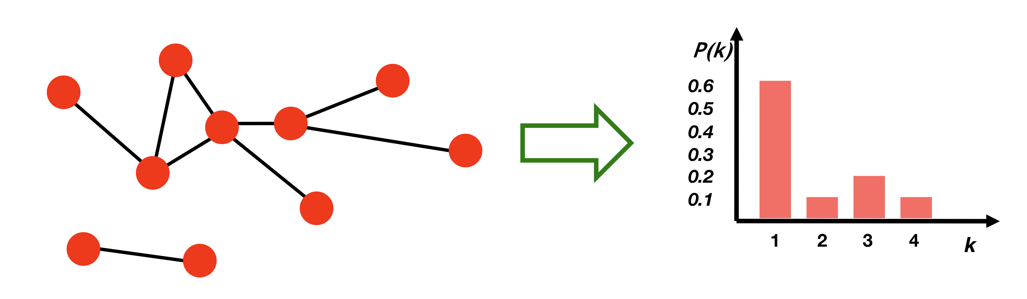
Degree distribution
임의로 선택된 node가 degree 를 갖을 확률
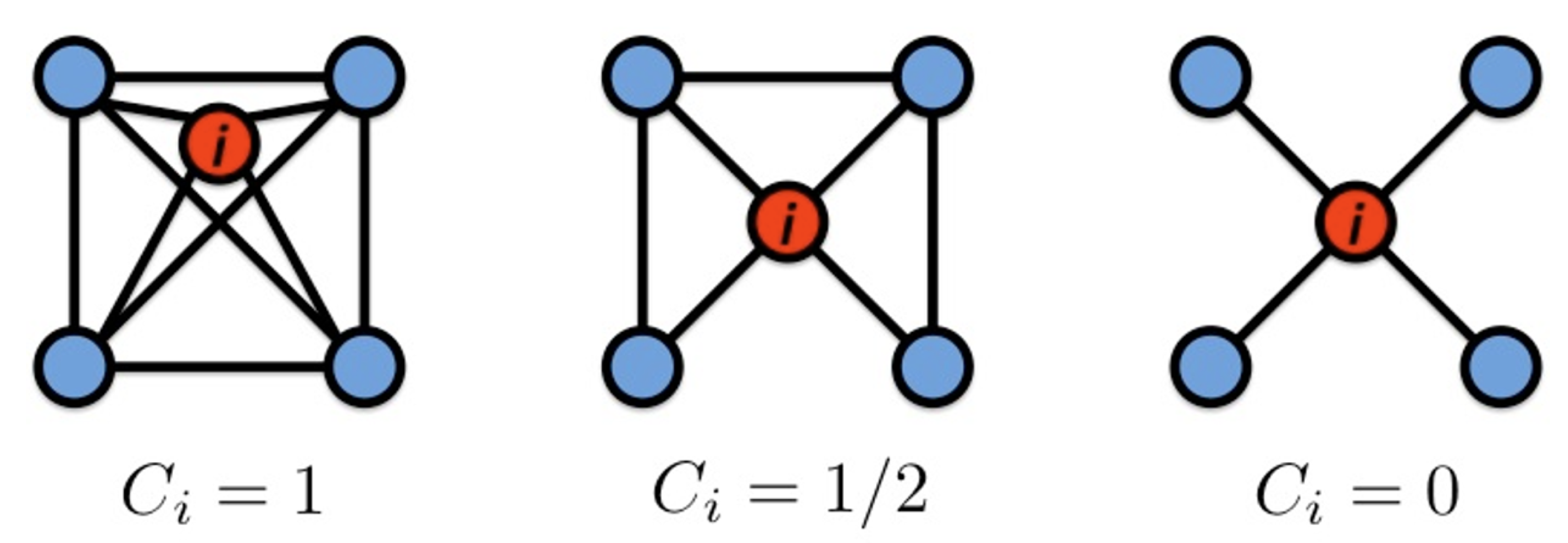
Clustering coefficient
node i의 이웃들이 연결된 정도
: node i 이웃들 사이의 edge들의 개수
: node i의 degree
cf)Graph Clustering coefficient: average over all the nodes clustering coefficient
Connectivity
가장 큰 연결된 component의 크기
component는 BFS를 이용해 찾는다.
Path Length
Diameter: 그래프 내 임의의 노드 쌍의 거리의 최대
Average path length
: node i와 node j의 거리
: 노드 쌍의 총합 =
Case Study
MSN graph를 통해 실제 그래프의 특성들을 확인하는 case study를 진행한다.
MSN은 Microsoft의 채팅 프로그램으로 communication network가 180M의 사람과 1.3B의 연결로 구성돼있다.
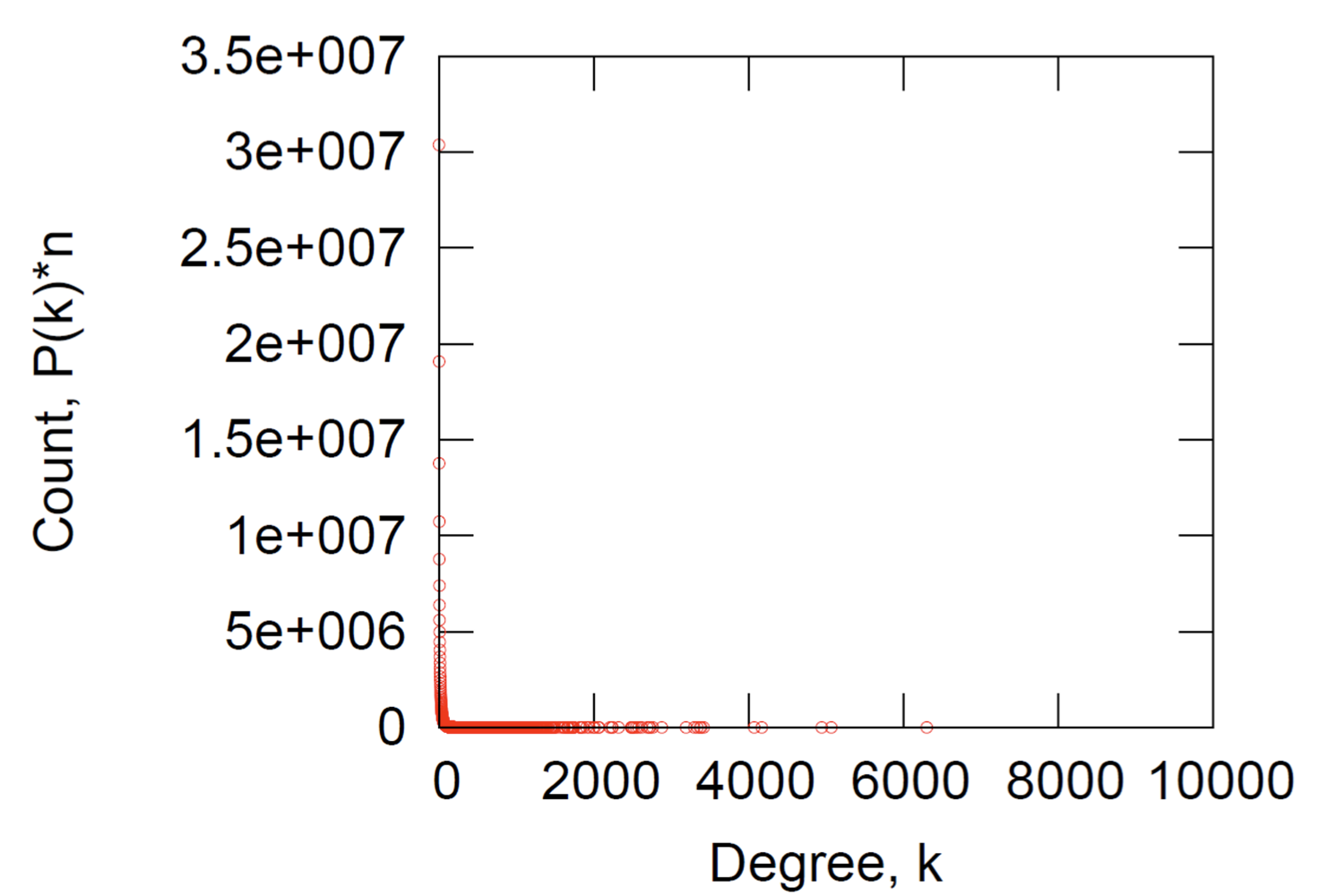
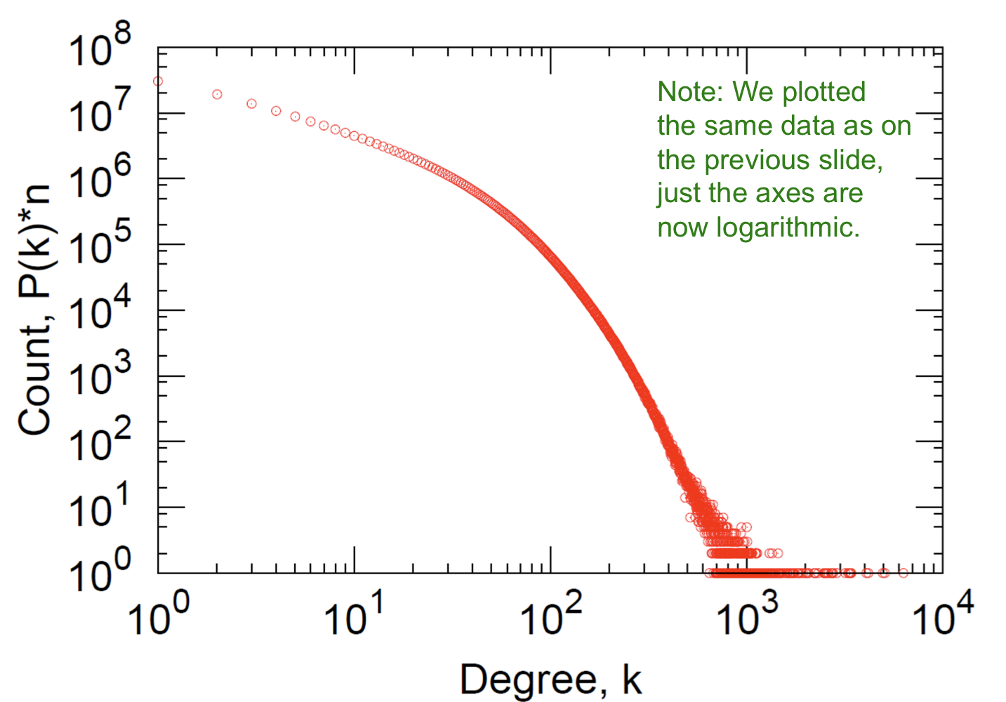
Degree Distribution
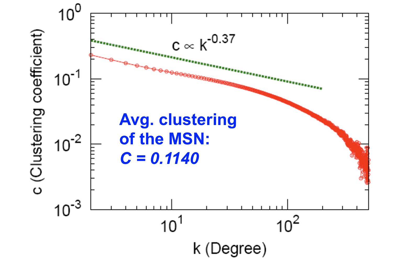
Clustering
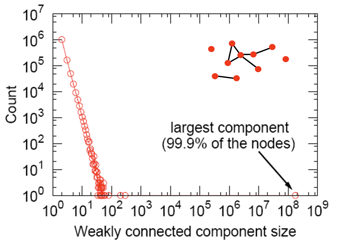
Connected Components
Path Length
Key Network Properties
- Degree distribution: avg.degree=14.4
- Clustering coefficient: 0.11
- Connectivity: giant component
- Path length: 6.6
Erdos-Renyi Random Graphs
- : undirected graph on n nodes where each edge (u,v) appears i.i.d. with probability p
- : undirected graph on n nodes, and m edges picked uniformly at random
우리는 를 다룬다.
Properties of
Degree Distribution
의 degree distribution은 이항분포(binomial)을 따른다.
n-1개에서 k개를 선택하여 k개는 p 확률로 연결되고, n-1-k개는 1-p 확률로 연결되지 않는다.
이항분포의 평균과 분산에 따라 다음을 알 수 있다.
- Mean
- Variance
Clustering Coefficient
: node i의 clustering coefficient
: node i의 이웃들간의 edge의 개수
: node i의 degree
의 edge들은 i.i.d. p 확률로 등장한다. 따라서 이를 통해 의 확률 분포를 알 수 있다.
이항분포의 기대값 공식을 통해
따라서 의 기대값을 다음과 같이 알 수 있다.
고정된 avg. degree에 대해 그래프의 크기를 키우면 C가 감소하는 것을 알 수 있다.
Connected Components
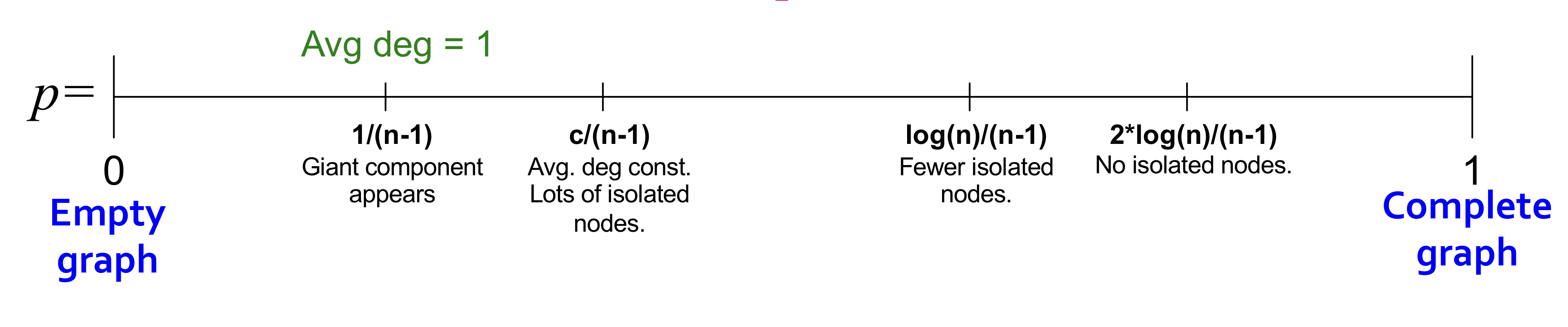
- Degree : all components are of size
- Degree : 1 ccomponent of size , others have size
Average degree가 1보다 클 때부터 Giant component가 등장한다. 따라서 k>1일 때, GCC가 존재한다.
Expansion
Definition
- Graph G(V,E) has expansion : if : the number of edges leaving
- =
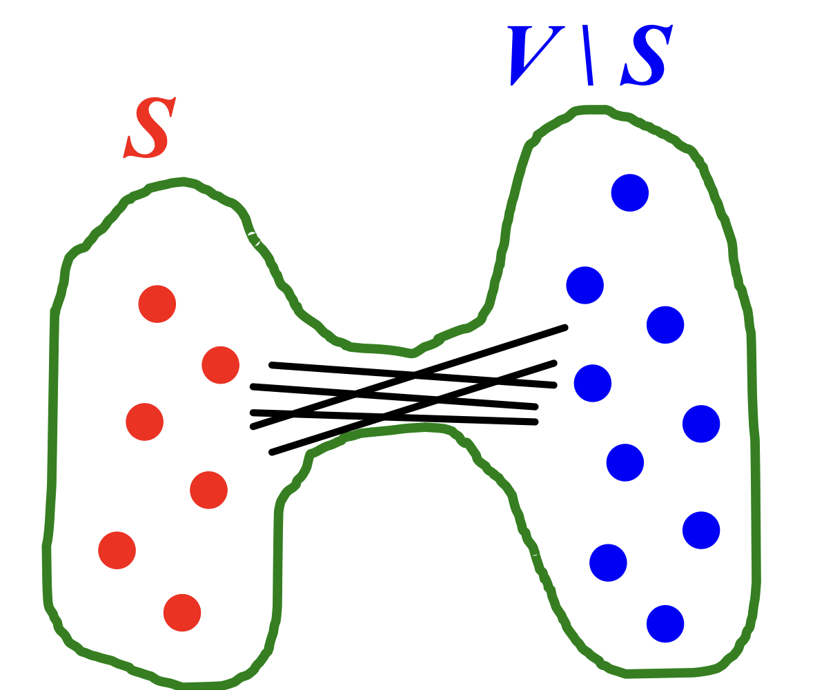
Expansion is measure of robustness.
이는 다음 그림을 통해 확인할 수 있다.
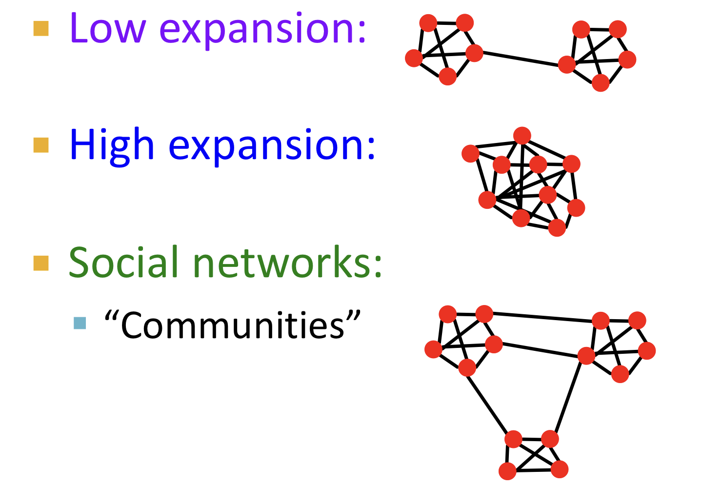
In a graph on n nodes with expansion for all pairs of nodes there is a path of length ).
- node의 개수가 많아지면 path length 증가한다.
- expansion 가 커지면 path length 감소한다.
For
- 랜덤 그래프들은 good expansion을 갖기 때문에 logarithmic number () 단계의 BFS로 모든 노드를 방문할 수 있다.
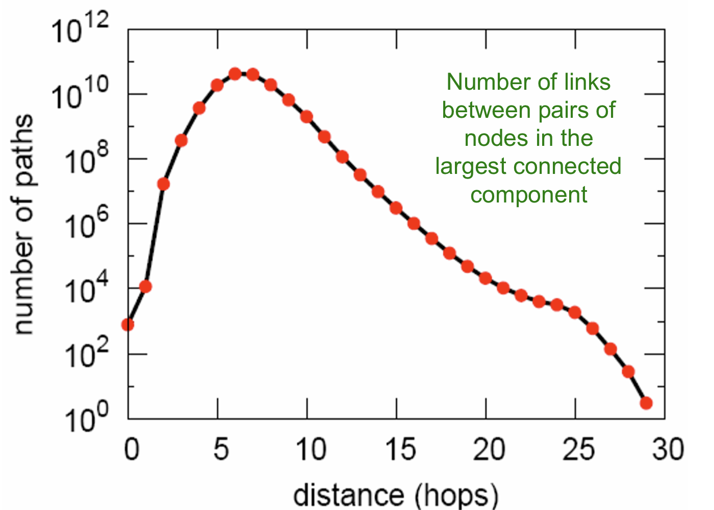
Shortest Path
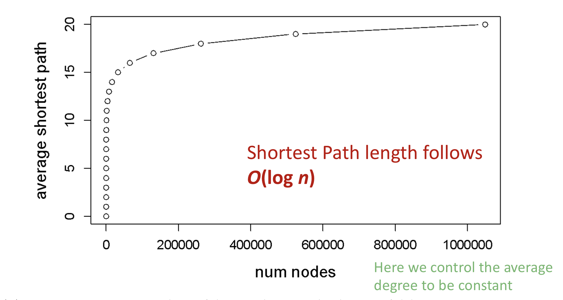
Erdos-Renyi random graph는 매우 커질 수 있지만, node들은 적은 hops 만큼 떨어져 있다.
위 그림에서 고정된 average degree에서 n에 따른 average shortest path가 logarithmic한 그래프를 그리는 것을 확인할 수 있다. 따라서 Erdos-Renyi random graph의 average shortest path는 .
Real Networks vs.
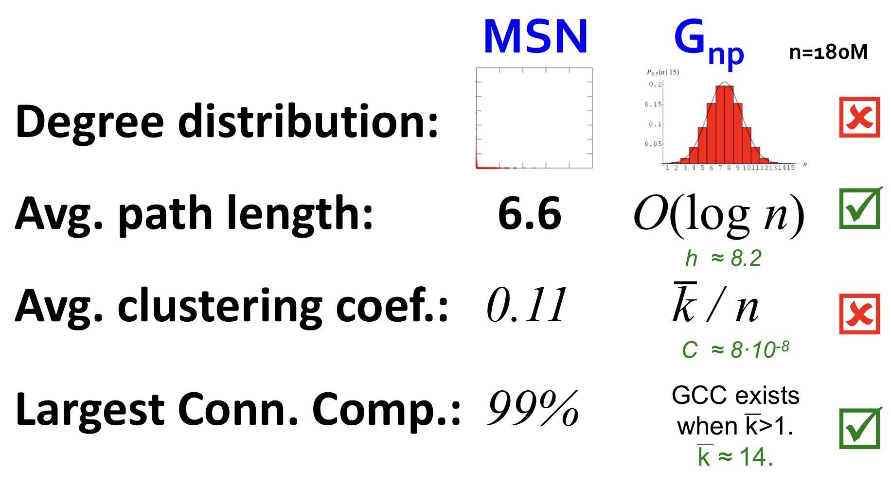
실제 그래프와 랜덤 그래프를 비교했을 때, clustering coefficient와 Degree distribution이 다른 것을 확인할 수 있다.
랜덤 네트워크 모델의 문제점들
- Degree distribution이 실제 네트워크와 다르다.
- 실제 네트워크 속의 Giant component는 phase transition을 통해 등장하지 않는다.
- 너무 낮은 clustering coefficient로 인해 local 구조가 없다.
phase transition: 직역 하자면 '단계 변이'이다. 랜덤 그래프에서 giant component는 average degree가 1 보다 큰 경우 등장한다. 즉, average degree가 1을 기준으로 단계가 나뉘어 giant component가 등장하는 것을 의미한다.
The Small-World Model
Motivation
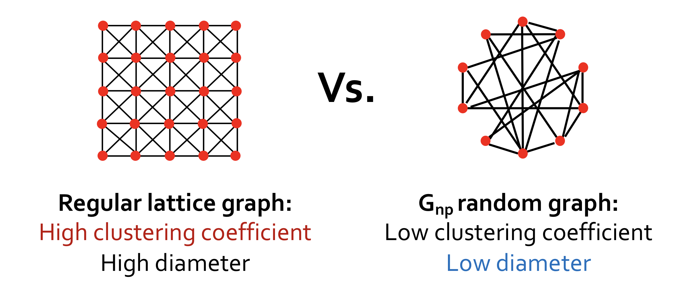
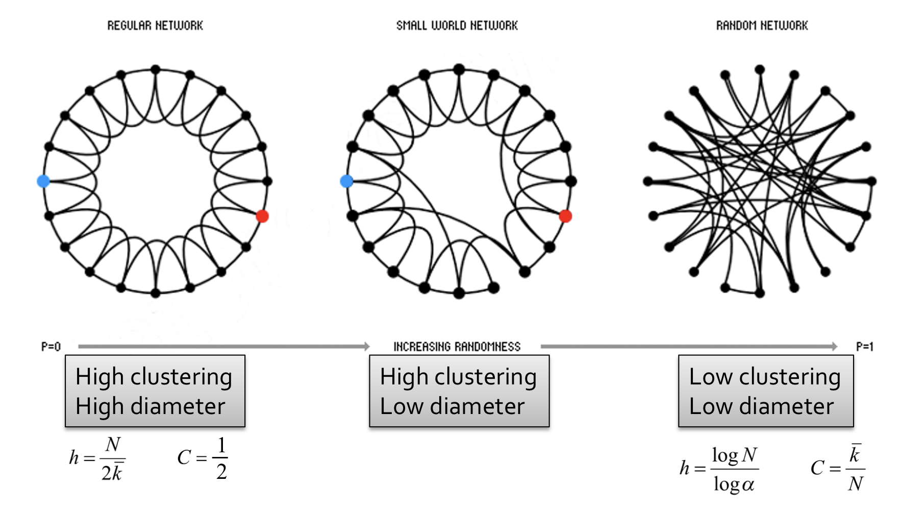
- Regular lattice graph: 높은 clustering coefficient와 높은 diameter를 갖는다.
- : 낮은 clustering coefficient와 낮은 diameter를 갖는다.
위의 그래프들과 다르게 실제 그래프는 local 구조를 갖고 있어 높은 clustering coefficient를 갖으면서 낮은 diameter를 갖는다.
MSN network는 대응되는 보다 7 order 큰 clustering을 갖는다. 다른 예시들은 다음과 같다.
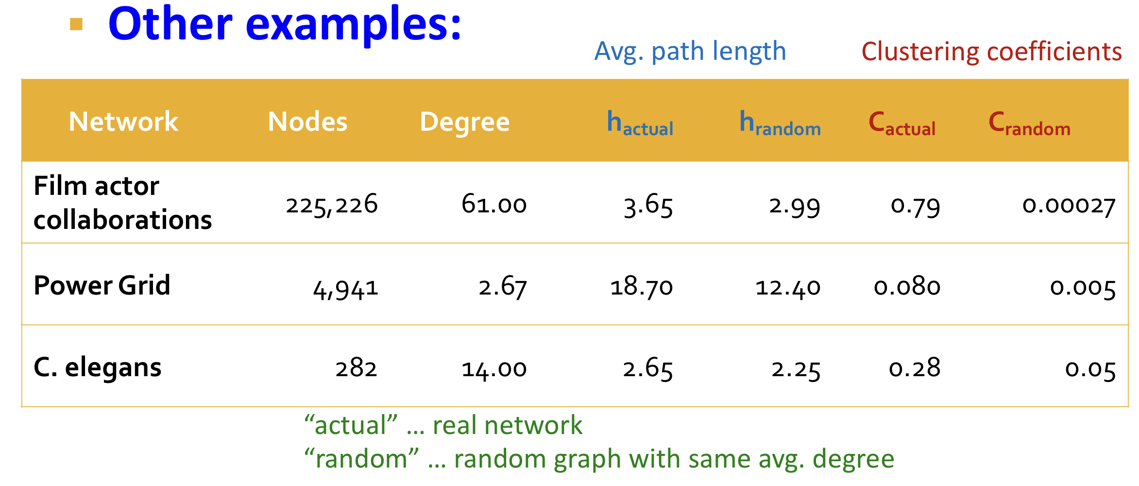
따라서 실제 그래프와 유사하게 high clustering coefficient를 갖으면서 low diameter를 갖고 싶다.
Idea
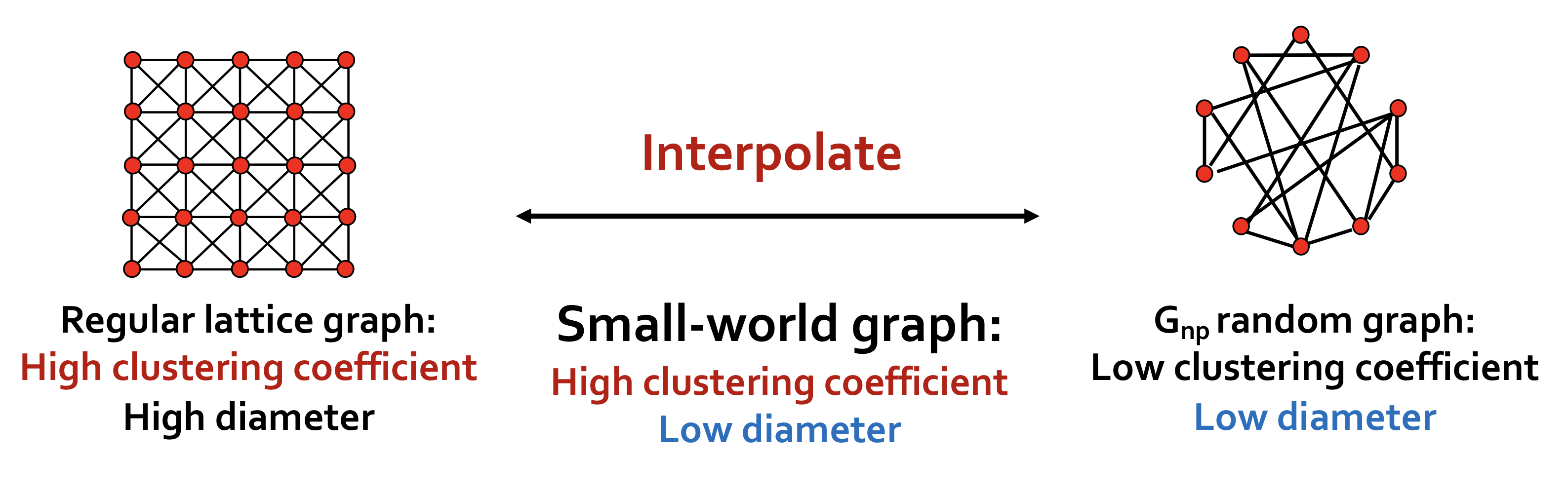
Regular lattice graphs와 를 interpolate(보간)하여 높은 clustering coefficient를 갖고 낮은 diameter를 갖는 Samll-world graph를 만든다.
Solution
(1) low-dimensional regular lattice
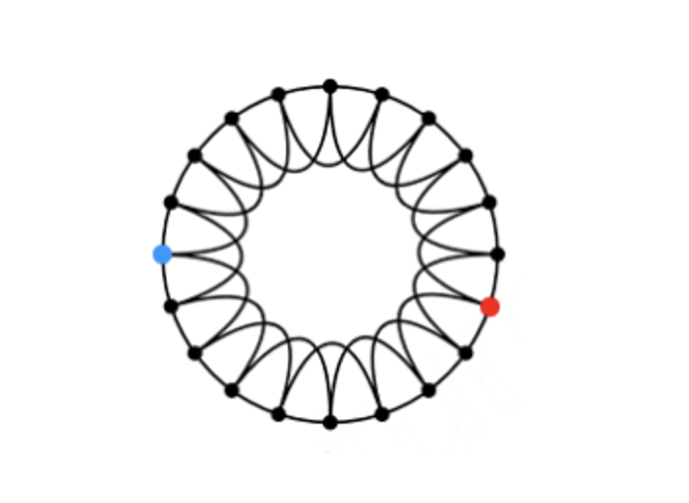
위 그림과 같이 이웃하는 노드와 2-hops인 노드를 이어 low-dimensional regular lattice를 만든다. (강의에서는 ring 모양을 활용)
- 높은 clustering coefficient와 높은 diameter를 갖는다.
(2) Rewire: Introduce randomness
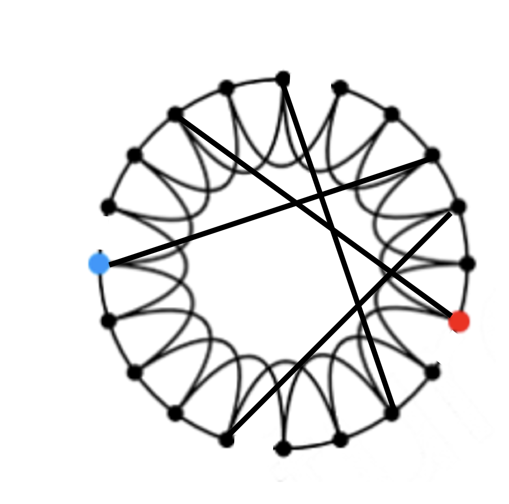
각각의 edge를 확률 p에 따라 임임의 노드로 endpoint를 옮긴다.
Rewiring을 통해 regular lattice와 random graph의 interpolate가 가능하다.
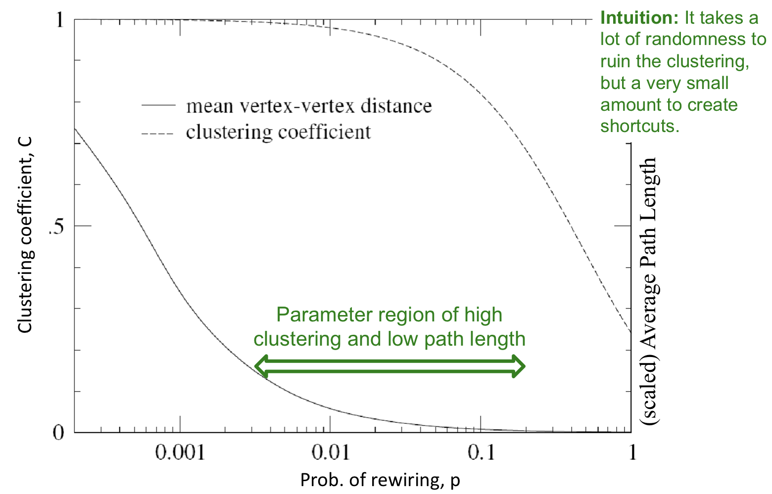
위의 그림과 같이 rewiring 확률 p가 특정 값들에 속할 때, 높은 clustering과 낮은 path length를 갖는 그래프를 생성할 수 있다.
Summary
- Clustering과 small-world 사이의 상호작용에 대한 insight를 제공
- 많은 실제 네트워크들의 구조를 포착
- 실제 네트워크들의 높은 clustering을 설명
- Degree distribution을 수정할 필요가 없다.
Kronecker Graph Model
Idea
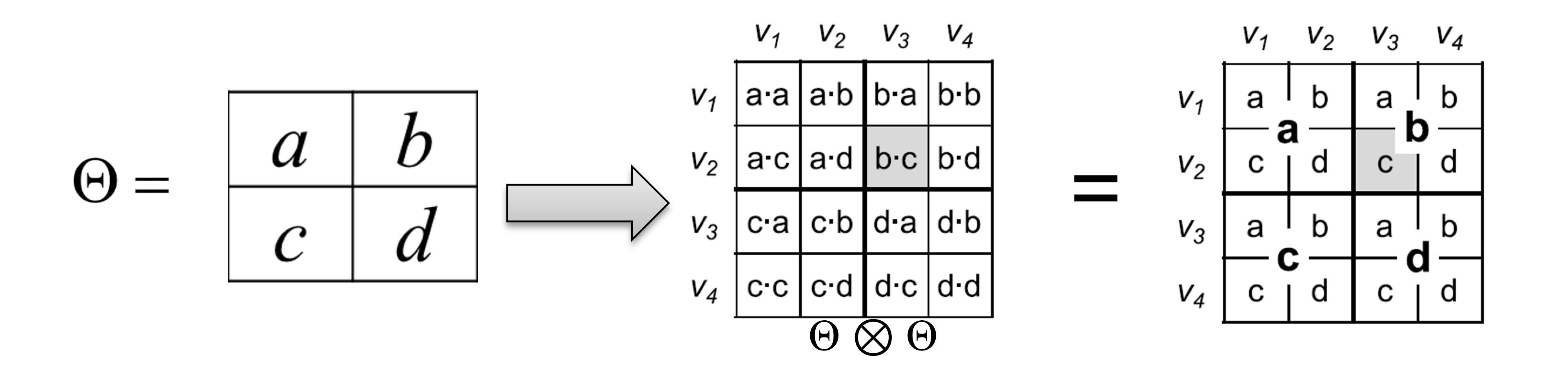
Self-similarity라는 직관을 이용해 재귀적인 그래프 구조를 생각한다. 따라서 재귀적으로 그래프 성장을 흉내낸다. 이를 위해 kronecker product를 이용한다. Kronecker product의 정의는 다음 그림과 같다.
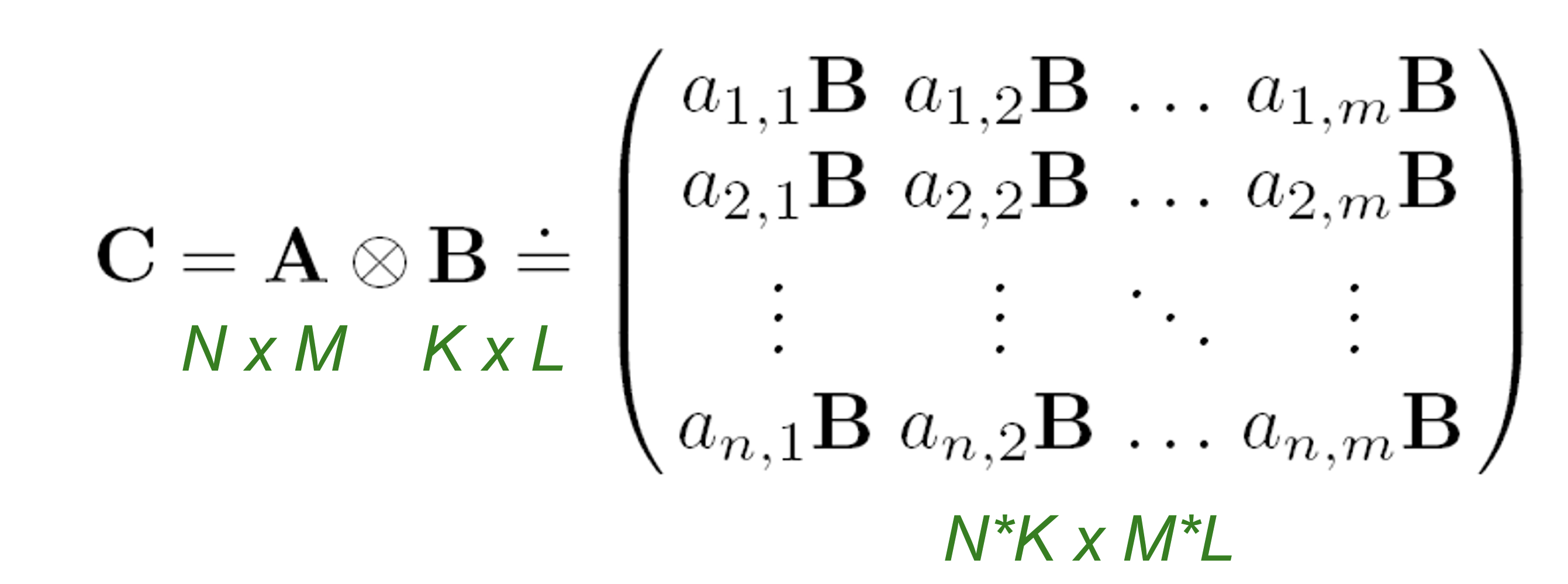
또한 두 그래프의 kronecker product를 그들의 인접행렬의 kronecker product로 정의한다.
Kronecker Graph
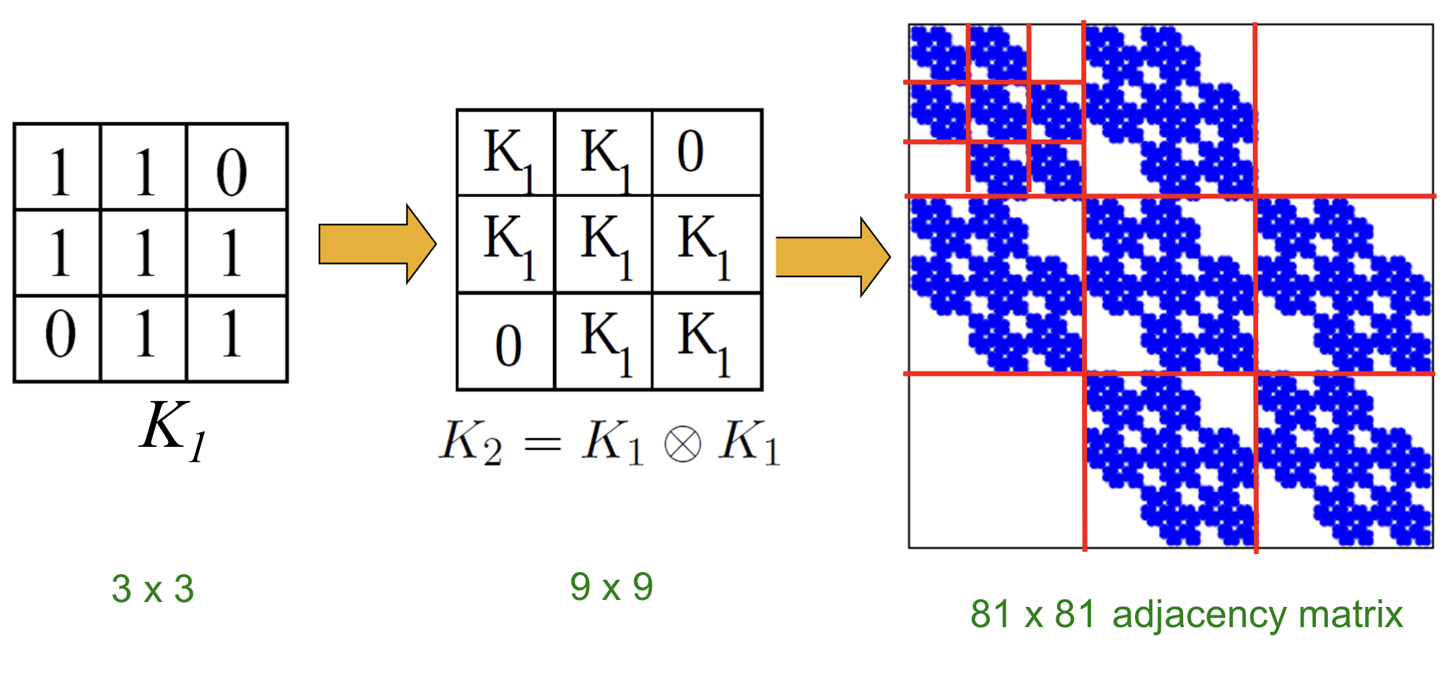
Kronecker graph는 초기 행렬 을 반복적으로 Kronecker product해서 얻을 수 있다.
Stochastic Kronecker Graphs
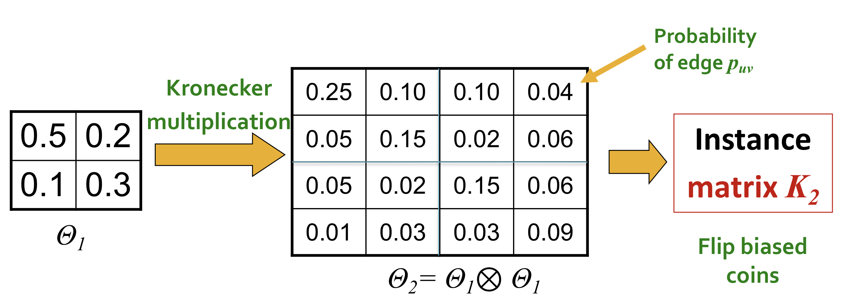
- 확률 행렬 를 생성
- Kronecker power 를 계산
- 의 확률에 따라 edge 를 생성해서 그래프 완성
위의 방법으로 stochastic Kronecker graph를 생성할 경우 의 복잡도를 갖게 된다. 즉, 노드의 개수에 따른 quadratic한 computational cost를 갖게 되므로 실제 적용하기엔 무리가 있다. 이를 해결하기 위해 Kronecker graph의 재귀적인 구조를 활용한 fast Kronecker graph generation algorithm이 존재한다.
Generation of Kronecker Graphs
-
먼저 normalized matrix L을 생성한다.
-
L의 확률에 따라 맨 오른쪽에 4분할된 영역에서 한 영역을 선택한다.
-
단계 2에서 선택된 영역에서 다시 2를 이용해 4분할된 영역 중에서 한 영역을 선택하고, 선택된 영역이 단일 cell이 될 때까지 반복한다.
-
선택된 단일 cell에 1을 할당한다. (즉, 연결됨을 의미) 선택된 단일 cell이 이전에 선택됬었으면 무시하고 진행한다.
-
단계 2,3,4를 최종 그래프의 기대 edge 개수인 E가 될 때까지 반복한다.
위의 알고리즘을 통해 의 computational cost로 Kronecker graph를 생성할 수 있다.
기대 edge 개수 E
E는 edge 개수의 기댓값이다. Stochastic Kronecker graph의 probability matrix의 cell은 각각 독립적인 베르누이 확률분포를 따르는 확률 변수이다. 베르누이 분포의 기대값은 확률 p 이고, 기대값의 선형성을 통해 probability matrix 노드 개수의 기대값을 덧셈을 통해 구할 수 있다.
위의 그림에 나오는 를 예시로 설명하면, 를 통해 생성된 Kronecker graph의 edge 개수는 a+b+c+d가 된다. Kronecker product를 m번 반복해서 생성된 probability matrix의 의 기대 edge 개수는 모든 cell의 값을 더하면 구할 수 있다. 또한 쉽게 각각의 cell들이 독립적인 확률변수라는 성질과 기대값의 성질을 이용하면 가 기대 edge 개수가 되는 것을 알 수 있다.
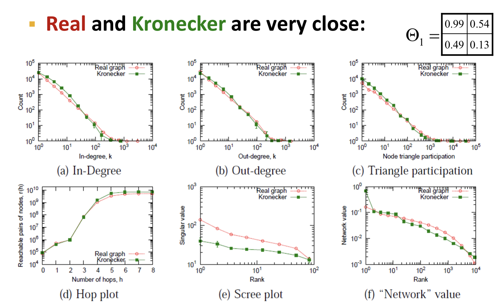
위의 그림을 통해 real graph와 Kronecker graph가 유사하다는 것을 알 수 있다.
References
- CS224W: Machine Learning with Graphs (Winter 2021) 14강
- Kronecker Graphs: An Approach to Modeling Networks 논문