작성자 : 투빅스 13기 이재빈
Contents
- Intro
- Shapley Value
- Additive Feature Attribution Method
- SHAP
- Code
Summary : SHAP 을 통해 Feature Attribution 을 파악할 수 있습니다.
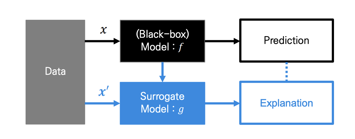
0. Intro
좋은 집을 찾고 있는 두빅스씨 ...
어떤 집 하나가 유난히 가격이 낮은데, 그 집이 숲 속에 있기 때문인지, 평수가 작기 때문인지, 혹은 평수가 작아 고양이를 기를 수 없어서 그렇기 때문인지 정확한 이유를 알 수 없습니다.
결과만 보고 해석하지 않고, 각 요소들이 결과값에 얼마나 영향을 미치는 지에 대해 파악하고자 합니다.
Limitations
기존의 Feature Attribution 파악 방법론에는 한계가 존재합니다.
1. Feature Importance
- Random Permutation 에 대해 Importance 를 측정하기 때문에, Inconsistent 합니다.
- Feature 간의 의존성 을 간과합니다.
설명변수 간 다중공선성이 존재하는 경우, 결과가 왜곡될 수 있습니다. - 음의 영향력 (-) 을 계산하지 않습니다.
모델이 negative feature 에 대한 학습을 의도적으로 무시하기 때문에, 에러가 높아지는 변인은 결과에 포함하지 않습니다.
2. PDP Plot
- 최대 3차원 까지만 표현 가능합니다.
비교하고자 하는 Feature 가 많아지면 시각화 할 수 없고, Feature 영향력이 과대 평가될 위험이 있습니다.
3. LIME
Global vs Local 대리 분석
- Global Surrogate Analysis
학습 데이터(일부 또는 전체)를 사용해 대리 분석 모델을 구축하는 것- Local Surrogate Analysis
학습 데이터 하나를 해석하는 과정
- Local Interpretable Model-agnostic Explanation
single prediction explanation 에 적합합니다. - Visualization 을 통한 결과 해석이 어렵습니다.
1. Shapley Value
Shapley Value 는 게임이론을 바탕으로, Game 에서 각 Player 의 기여분을 계산하는 방법입니다.
✔︎ Game Theory
개인 또는 기업이 어떠한 행위를 했을 때, 그 결과가 게임에서와 같이 자신뿐만 아니라 다른 참가자의 행동에 의해서도 결정되는 상황에서, 자신의 최대 이익에 부합하는 행동을 추구한다는 수학적 이론✔︎ 협력적 게임 이론 (Cooperative Game Theory)
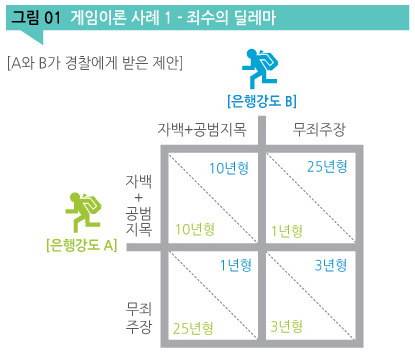
비협력적으로 게임을 했을 때 각 개인이 취하는 이득보다, 협력적으로 게임을 했을 때의 각 개인이 취하는 이득이 더 크다면, 긍정적인 협동이 가장 최선의 선택지대표적인 예시 : 죄수의 딜레마
하나의 특성에 대한 중요도를 알기 위해 → 여러 특성들의 조합을 구성하고 → 해당 특성의 유무에 따른 평균적인 변화를 통해 값을 계산합니다.
- : 데이터에 대한 Shapley Value
- : 전체 집합
- : 전체 집합에서, 번째 데이터가 빠진 나머지의, 모든 부분 집합
- : 번째 데이터를 포함한 (=전체) 기여도
- : 번째 데이터가 빠진, 나머지 부분 집합의 기여도
Example
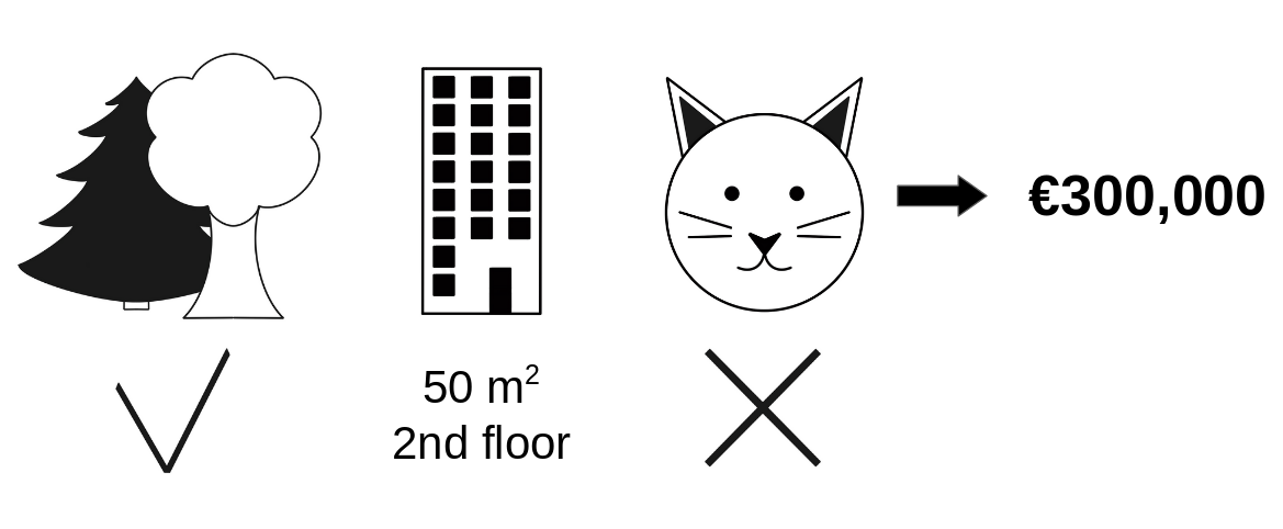
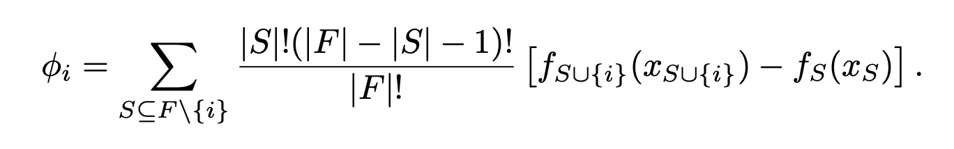
집값을 결정짓는 요인으로, [숲세권, 면적, 층, 고양이 양육 가능 여부] 등의 Feature 가 존재합니다.
'고양이 양육 가능 여부' 의 집값에 대한 기여분은, 그 외 모든 Feature 가 동일하다는 가정 하에,
310,000 (고양이 함께 살기 불가능) - 320,000 (고양이 함께 사는 것 가능) = -10,000 으로 계산됩니다.
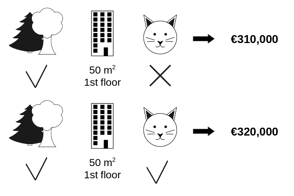
이러한 과정을 모든 가능한 조합에 대해 반복합니다.
[숲세권, 면적, 층, 고양이 양육 가능 여부] : 4개
= 8 개의 조합이 존재하며, 8개의 조합에 각각에 대해
{f(조합1 😺) - f(조합1)} + ... + {f(조합8 😺) - f(조합8)} 값을 산출하고, 이를 가중평균 하여 (😺) 를 구합니다.
Classic Shapley Value Estimation
- consistency : 매 회 계산할 때 마다 같은 결과를 출력합니다.
- multicollinearity : 서로 영향을 미칠 가능성을 고려합니다.
- Feature Importance 가 고려하지 못하는, 음의 영향력을 고려할 수 있습니다.
2. Additive Feature Attribution Method
Definition
Additive Feature Attribution Methods have an explanation model that is a linear function of binary variables :
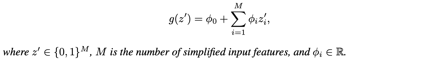
- : explanation model ,
- : original prediction model
- : simplified input ,
- : mapping function ,
- : attribution value
ex. LIME, DeepLIFT, Layer-Wise Relevance Propagation, Shapley Value
복잡한 모델 대신, 해석이 간단한 모델 로 해석하고자 합니다.
는 복잡한 모델에 특화되어 있는, 복잡한 데이터입니다.
따라서 의 해석 용이성을 위해 간단화 된 변수 를 사용하고자 하며,
Simplified input 는 라는 mapping function 으로 정의됩니다.
라는 가정을 통해, 으로 표현되며,
(1 : input is included in the model / 0 : excluded)
가 되도록 Surrogate Model 은 학습됩니다.
✔︎ Additive Feature Attrbution
원래의 input 가 아닌, Simplified input 를 통해,
를 만족하는 Explanation Model 를 만드는 방법입니다.
Properties
✔︎ Desirable Properties
Feature Attribution 은 1. Local Accuracy, 2. Missingness, 3. Consistency 특성 모두를 만족하기를 원합니다.
1. Local Accuracy
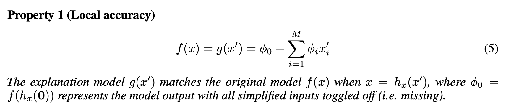
simplified input 를 explanation model 에 넣었을 때의 output 는, original input 에 대한 와 match 가 잘 되어야 합니다.
✓ (Efficiency) 각 팀원 점수를 합치면, 전체 점수가 되어야 합니다.
2. Missingness
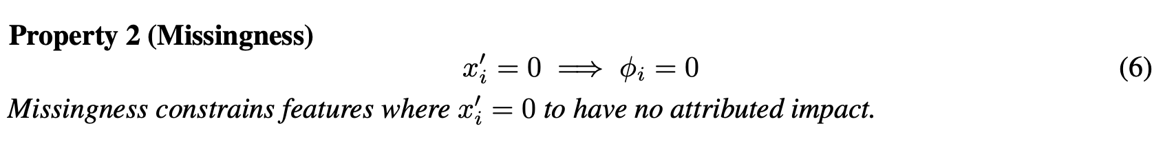
Feature 값이 없다면, Attribution 값도 0이 되어야 합니다.
✓ 팀플에 참여하지 않았다면, 개인 점수는 0점이 되어야 합니다.
3. Consistency
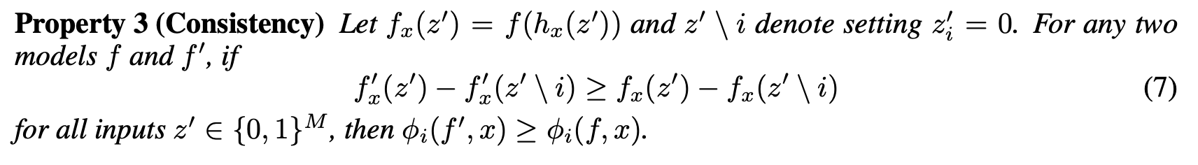
모델이 변경되어 Feature 의 Marginal Contribution 이 (다른 특성에 관계없이) 증가하거나 동일하게 된다면, Attribution 도 증가하거나 동일하게 유지되어야 하며, 감소할 수 없습니다.
✓ 매번 똑같은 방식으로 play 했다면, 결과 점수가 똑같아야 합니다.
Theorem
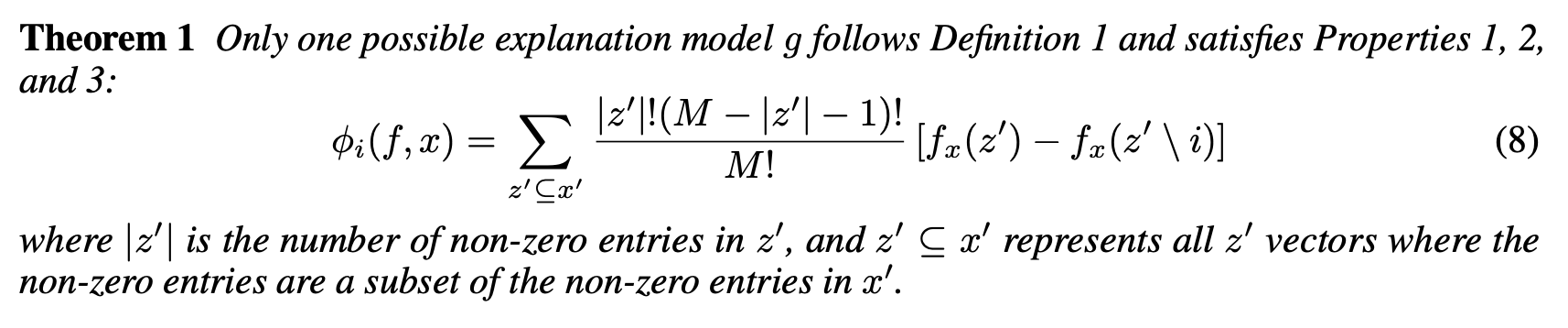
Additive Feature Attribution 의 정의와 3가지 Desired Properties 를 만족하는 유일한 방법은, Theorem1 수식입니다.
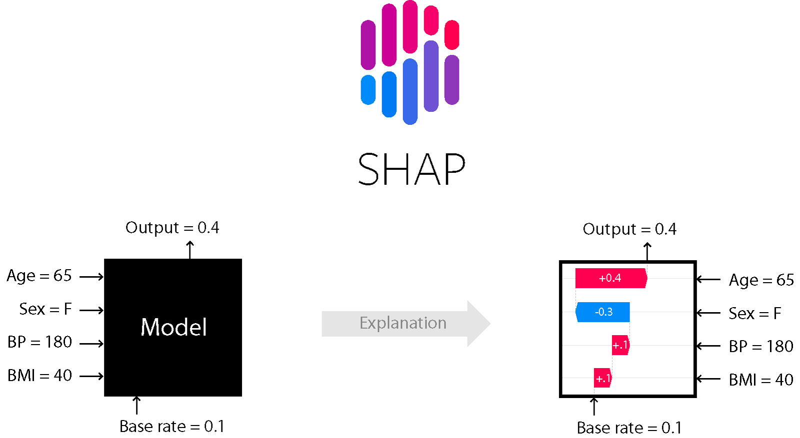
SHAP = Shapley Value 를 사용하여, Additive Method 를 만족시키는 Explanation Model
3. SHAP
SHAP : Shapley Value 의 Conditional Expectation
Simplified Input을 정의하기 위해 정확한 값이 아닌, 의 Conditional Expectation을 계산합니다.
오른쪽 화살표 () 는 원점으로부터 가 높은 예측 결과를 낼 수 있게 도움을 주는 요소이고, 왼쪽 화살표 () 는 예측에 방해가 되는 요소입니다.
- SHAP은 Shapley Value (Local Explanation) 기반으로 하여, 데이터 셋의 전체적인 영역을 해석이 가능합니다. (Global Surrogate)
- 모델 의 특징에 따라, 계산법을 달리하여 빠르게 처리합니다.
- Kernel SHAP : Linear LIME + Shapley Value
- Tree SHAP : Tree based Model
- Deep SHAP : DeepLearning based Model
Kernel SHAP
instance 에 대한 explanation 을 구합니다.
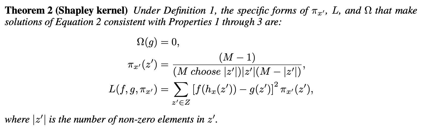
- Feature value 에서, 조합을 생성합니다.
단, 를 그대로 사용하지 않고, 로 사용하는, Random Feature Coalition 을 생성합니다. - 인 경우 actual feature value 에 mapping 되고,
인 경우 random sample value 로 mapping 됩니다.
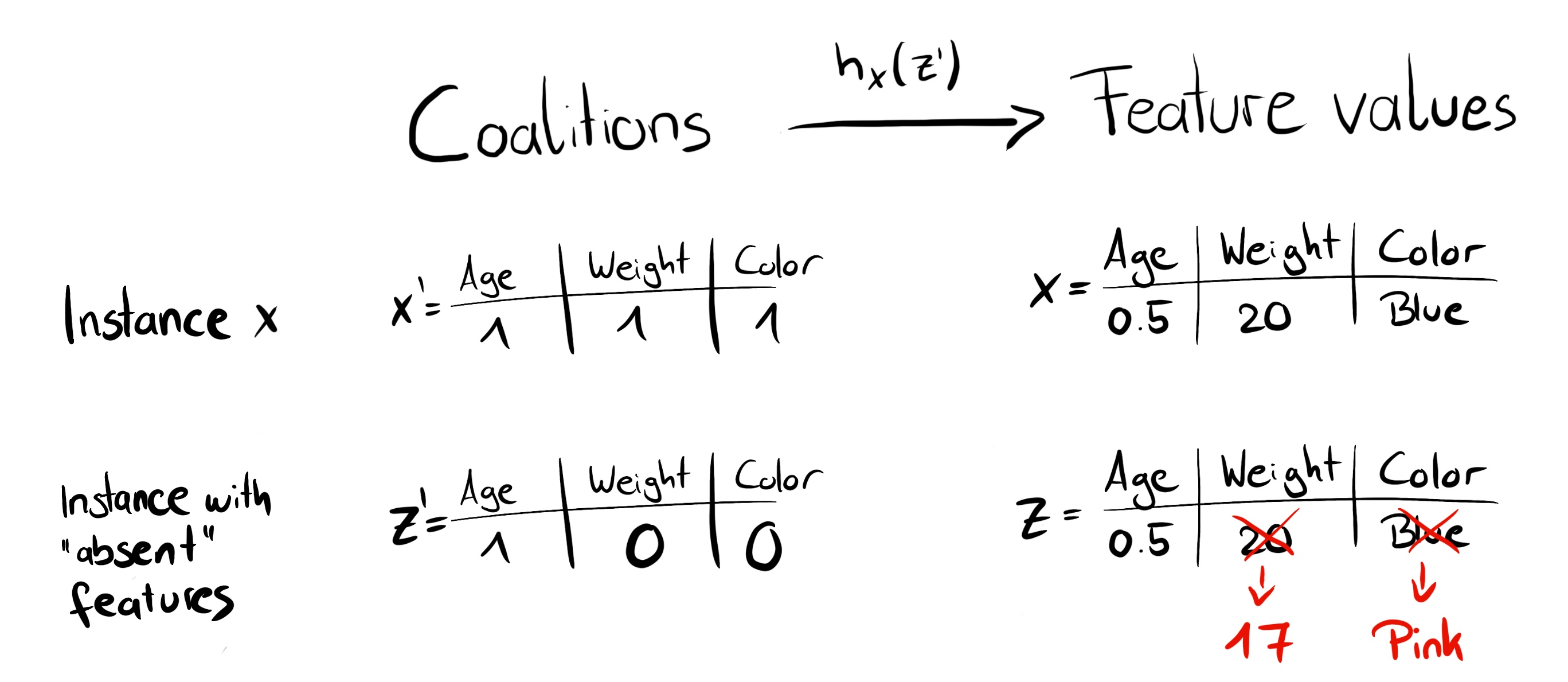
- 를 본래의 feature space 로 mapping 시킨 다음, 모델 에 적용함으로써, 예측값을 얻습니다.
즉, Local Surrogate Model 에 대한 설명변수는 0과 1로 이루어진 값이 되며, 반응변수는 이에 대한 예측값이 됩니다. - 각 Feature 조합마다 SHAP Kernel 을 적용하여, Weight 를 계산해 Linear Model 를 적합시킵니다.
- Linear Model 로 부터 계수값인 = Shapley Value 를 반환합니다.
Tree SHAP
Tree Ensemble Model 의 Feature Importance 는 모델(or 트리)마다 산출값이 달라지기 때문에, Inconsistent 하다는 한계점이 존재합니다.
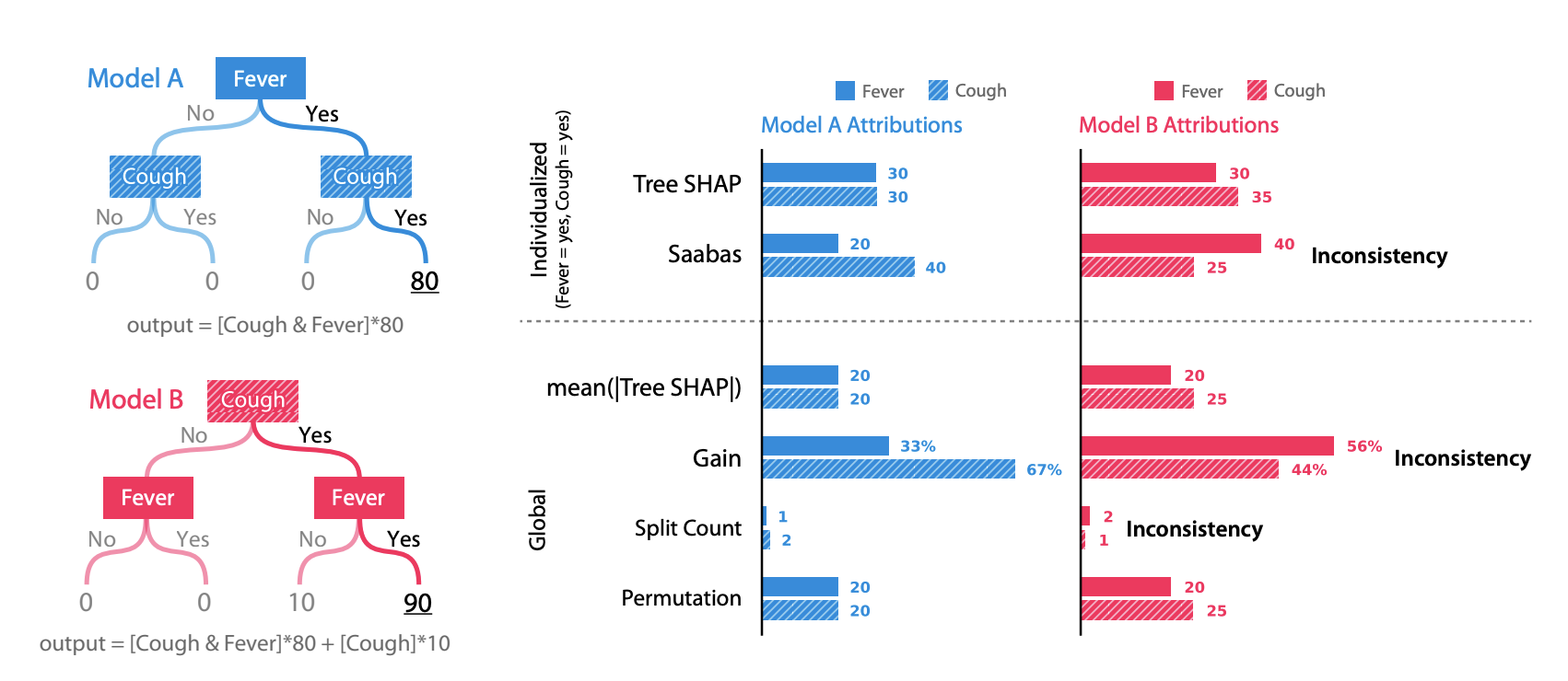
Tree Model A 와 B 의 Feature 는 Fever, Cough 로 동일하지만, split 순서가 다릅니다. Split 순서에 기반하여 계산되는 Gain, Split Count 등의 산출값이 달라지는 것을 확인할 수 있습니다.
즉, 같은 데이터로부터 학습이 된 모델이지만, 모델마다 Feature Importance 가 달라지게 됩니다.
SHAP 은 Split 순서와 무관하게, Consistent 한 Feature Importance 를 계산할 수 있습니다.
= 가 속하는 Leaf node의 score 값 해당 node에 속하는 Training 데이터의 비중
각 Tree 마다 Conditional Expectation 를 구해, 다 더하여 최종 값을 산출합니다.
시간복잡도 :
T : 트리의 개수, L : 모든 트리의 최대 leaf 수, D : 모든 트리의 최대 깊이
Kernel SHAP 에 비해 속도가 빠릅니다.
4. Code
1. Tree SHAP
# import packages
import pandas as pd
import numpy as np

from xgboost import XGBRegressor, plot_importance
from sklearn.model_selection import train_test_split

import shap

# load data
X, y = shap.datasets.boston()
X_train, X_test, y_train, y_test = train_test_split(X, y, test_size=.2, random_state=1)

# modeling
model = XGBRegressor()
model.fit(X_train, y_train)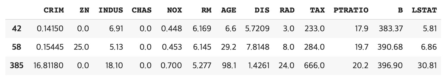
보스턴 주택 가격 데이터를 통해, 집값을 결정짓는 요인에 대해 알아봅니다.
XGBoost Regressor 로 집값을 예측하는 모델을 만들고, SHAP value 를 통해 Feature Attribution 을 파악합니다.
0. Load SHAP
# load js
shap.initjs()

'''
KernelExplainer() : KNN, SVM, RandomForest, GBM, H2O
TreeExplainer() : tree-based machine learning model (faster)
DeepExplainer() : deep learning model
'''

explainer = shap.TreeExplainer(model)
shap_values = explainer.shap_values(X_train)
1. force_plot
특정 데이터 하나 & 전체 데이터에 대해, Shapley Value 를 1차원 평면에 정렬해서 보여줍니다.
# 첫 번째 데이터에 대한 SHAP 시각화
shap.initjs()
shap.force_plot(explainer.expected_value, shap_values[0,:], X_train.iloc[0,:])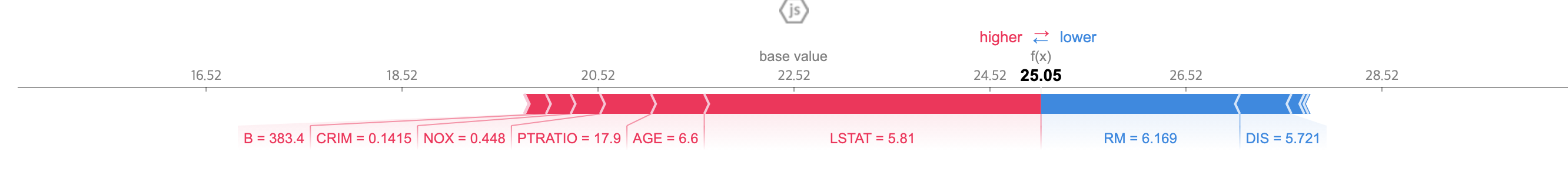
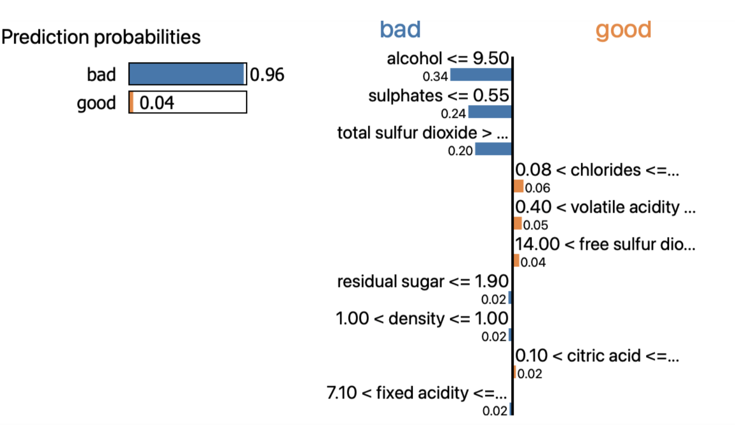
특정 데이터 (궁금한 어떤 주택)에 대한 Shapley value 를 분해하고 시각화합니다.
집값 상승에 긍정적인 영향을 준 요인은 LSTAT (동네의 하위 계층 비율) 이며, 부정적인 영향을 준 요인은 RM (방의 수) 입니다.
비슷한 조건의 다른 주택에 비해 방의 수 요인이 집값 형성에 부정적인 영향을 미쳤다고 해석할 수 있습니다.
# Outlier 에 대한 SHAP 시각화
shap.initjs()
shap.force_plot(explainer.expected_value, shap_values[259,:], X_train.iloc[259,:])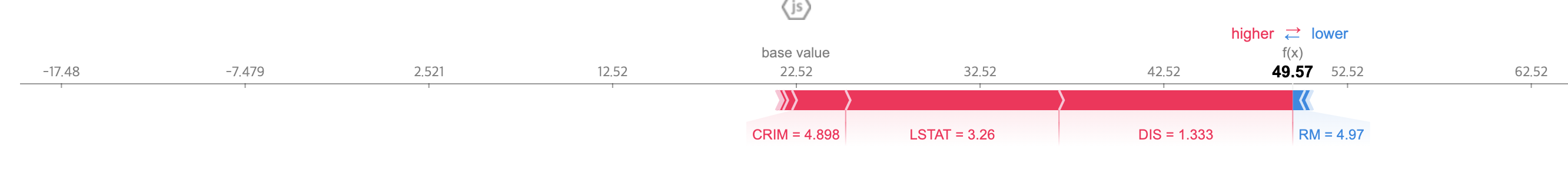
주요 업무지까지 거리가 가깝고 (DIS), 주변 지역에 하위 계층 사람들이 적게 살면서 (LSTAT), 범죄율이 극도로 낮으므로 (CRIM), 주택 자체의 상태보다 주변 환경에 의해 좋은 집값이 형성되었음을 알 수 있습니다.
# 전체 데이터에 대한 SHAP 시각화
shap.initjs()
shap.force_plot(explainer.expected_value, shap_values, X_train)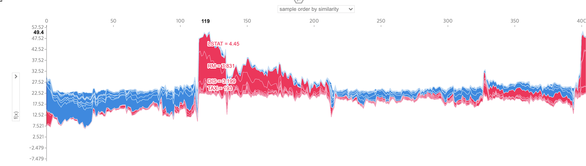
전체 데이터에 대해 Shapley Value를 누적하여 시각화 할 수 있으며, 이를 기반으로 Supervised Clustering 또한 진행할 수 있다고 합니다.
Feature 하나에 대한 전체 누적 Shapley Value 를 구할 수 있습니다.
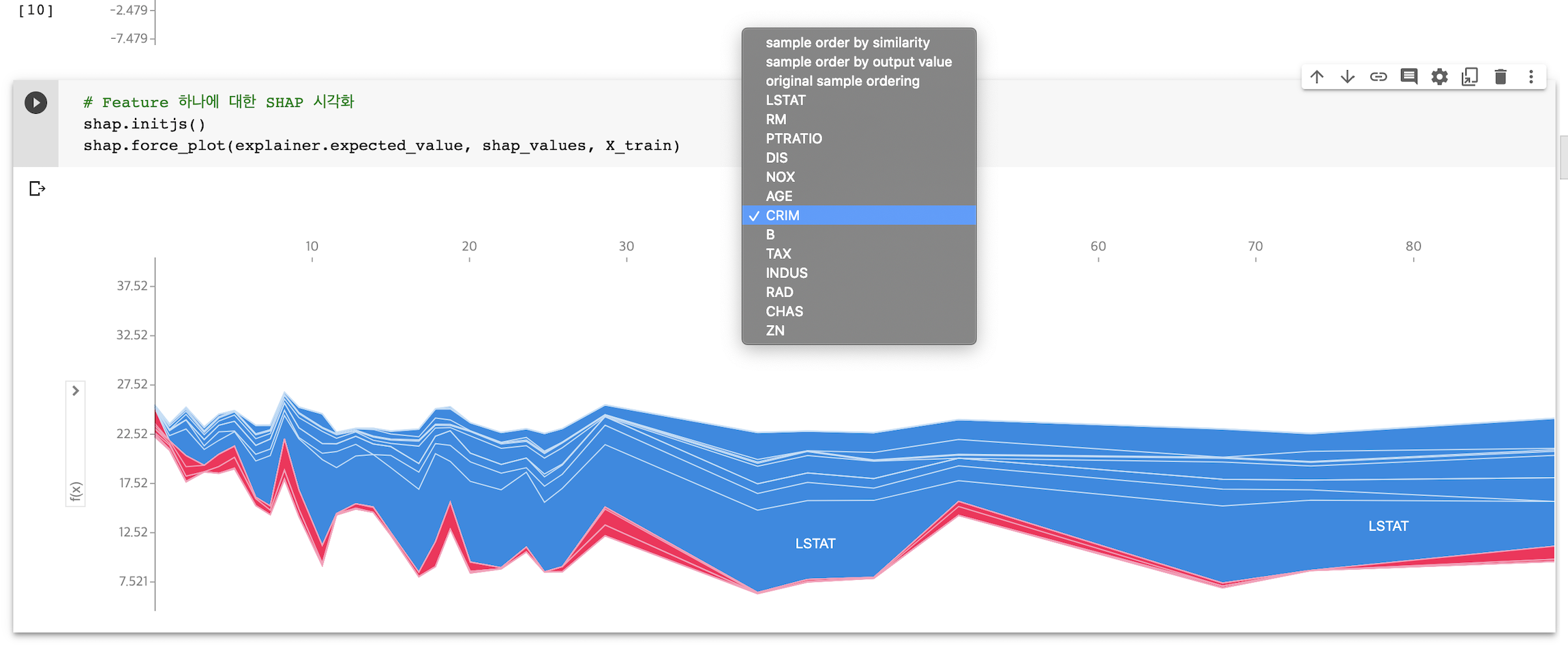
2. dependence_plot
Feature 하나에 대한 SHAP 영향력을 보여줍니다.
shap.initjs()
top_inds = np.argsort(-np.sum(np.abs(shap_values), 0))  # (13, ) : 각각의 Feature 에 대해 shap value 다 더한 것

# make SHAP plots of the three most important features
for i in range(2):
    shap.dependence_plot(top_inds[i], shap_values, X_train)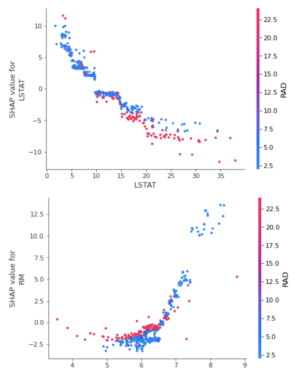
위의 코드는 영향력이 큰 변수들 순서대로 출력하는 방법이며, top_inds[i] 에 특정 Feature 를 넣어 영향력을 파악할 수 있습니다.
3. summary_plot
shap.summary_plot(shap_values, X_train)
전체 Feature 들이 Shapley Value 분포에 어떤 영향을 미치는지 시각화 할 수 있습니다.
shap.summary_plot(shap_values, X_train, plot_type='bar')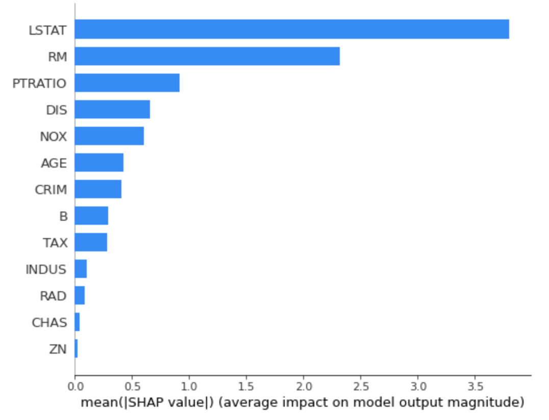
각 Feature 가 모델에 미치는 절대 영향도를 파악할 수 있습니다.
4. interaction plot
shap_interaction_values = shap.TreeExplainer(model).shap_interaction_values(X_train)

# main effect on the diagonal
# interact effect off the diagonal
shap.summary_plot(shap_interaction_values, X_train)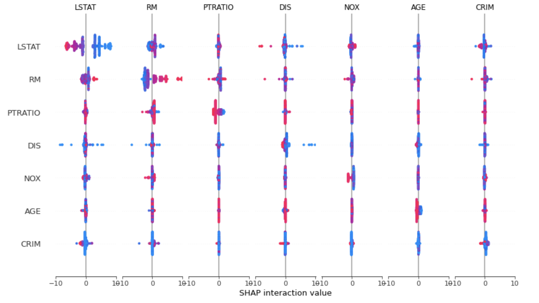
Feature 사이의 interaction 또한 파악할 수 있습니다.
shap.dependence_plot(
    ("RM", "LSTAT"),
    shap_interaction_values, X_train,
    display_features=X_train
)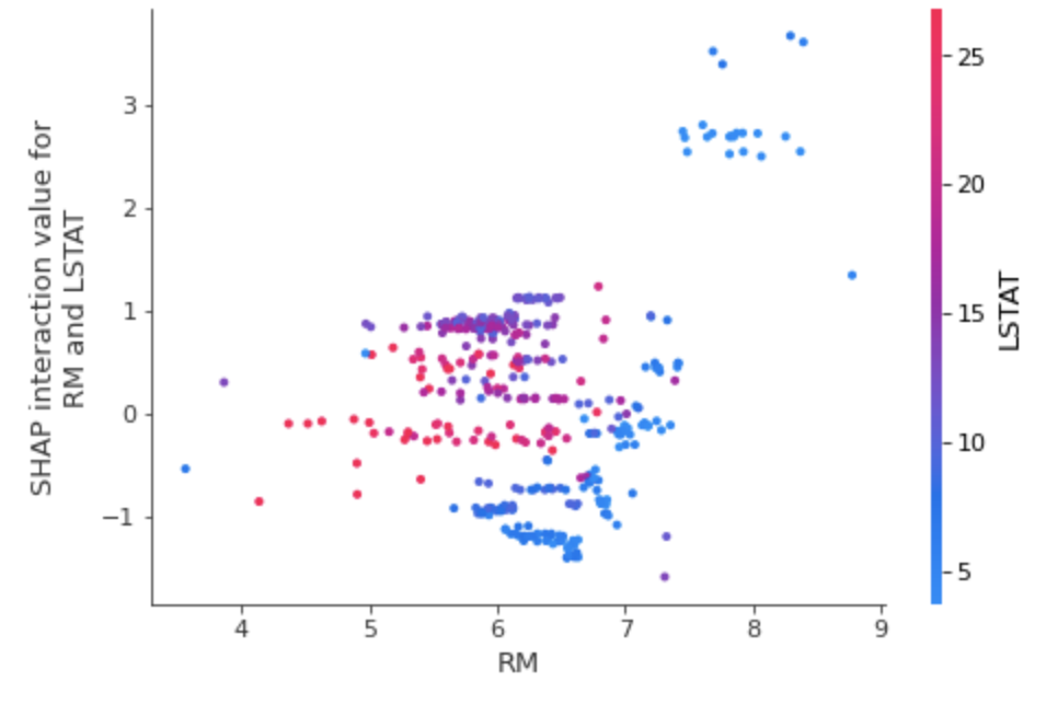
dependency_plot 을 통해 두 개 변수 사이의 영향력 시각화 가능합니다.
영향력 분해 또한 가능하다고 합니다.
(출처 : Explainable AI for Trees: From Local Explanations to Global Understanding)
2. Deep SHAP
1. NLP
import transformers
transformer = transformers.pipeline('sentiment-analysis', return_all_scores=True)

explainer2 = shap.Explainer(transformer)
shap_values2 = explainer2(["What a great movie! ...if you have no taste."])

shap.plots.text(shap_values2[0, :, "POSITIVE"]) 
2. DeepSHAP
import tensorflow as tf

# 1. dataset 불러오기
mnist = tf.keras.datasets.mnist
(x_train, y_train), (x_test, y_test) = mnist.load_data()
x_train, x_test = x_train / 255.0, x_test / 255.0  # image scaling : (0,1) 범위로 바꿔주기

# 2. model 구성하기
model = tf.keras.models.Sequential([
  tf.keras.layers.Flatten(input_shape=(28, 28)),
  tf.keras.layers.Dense(128, activation='relu'),
  tf.keras.layers.Dropout(0.2),
  tf.keras.layers.Dense(10, activation='softmax')
])

# 3. model 학습과정 설정하기
model.compile(optimizer='adam',
              loss='sparse_categorical_crossentropy',
              metrics=['accuracy'])

# 4. model 학습
model.fit(x_train, y_train, epochs=3)
# select a set of background examples to take an expectation over
background = x_train[np.random.choice(x_train.shape[0], 100, replace=False)]
# explain predictions of the model on four images
e = shap.DeepExplainer(model, background)
# ...or pass tensors directly
# e = shap.DeepExplainer((model.layers[0].input, model.layers[-1].output), background)
shap_values = e.shap_values(x_test[:5])
# plot the feature attributions
shap.image_plot(shap_values, -x_test[:5])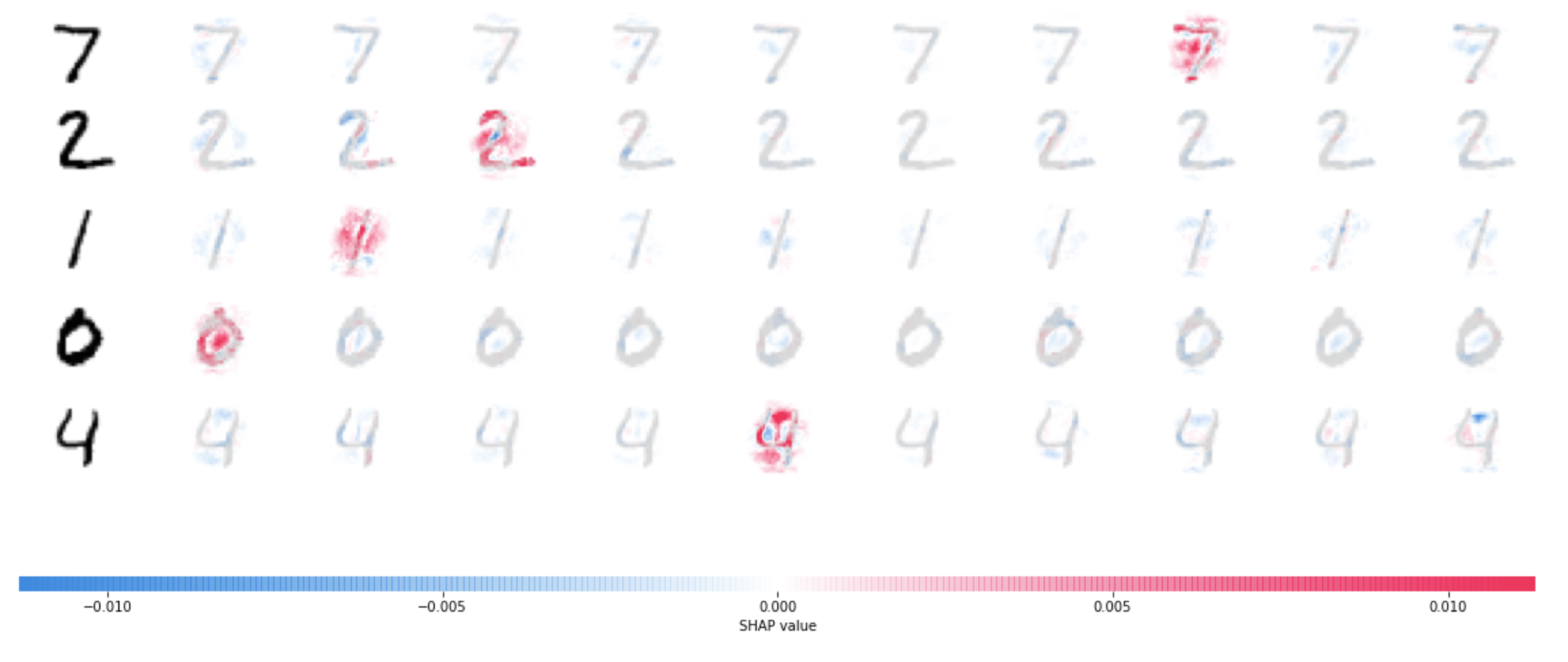
mnist classification 에 대한 SHAP 시각화 결과입니다.
4 와 9 를 예측함에 있어서 - 부분이 핵심적인 역할을 한다고 해석할 수 있습니다.
3. GradientExplainer
from keras.applications.vgg16 import VGG16
from keras.applications.vgg16 import preprocess_input
import tensorflow.python.keras.backend as K
import json

# load pre-trained model and choose two images to explain
model = VGG16(weights='imagenet', include_top=True)
X,y = shap.datasets.imagenet50()
to_explain = X[[39,41]]

# load the ImageNet class names
url = "https://s3.amazonaws.com/deep-learning-models/image-models/imagenet_class_index.json"
fname = shap.datasets.cache(url)
with open(fname) as f:
    class_names = json.load(f)

# explain how the input to the 7th layer of the model explains the top two classes
def map2layer(x, layer):
    feed_dict = dict(zip([model.layers[0].input], [preprocess_input(x.copy())]))
    return K.get_session().run(model.layers[layer].input, feed_dict)
e = shap.GradientExplainer(
    (model.layers[7].input, model.layers[-1].output),
    map2layer(X, 7),
    local_smoothing=0 # std dev of smoothing noise
)
shap_values,indexes = e.shap_values(map2layer(to_explain, 7), ranked_outputs=2)

# get the names for the classes
index_names = np.vectorize(lambda x: class_names[str(x)][1])(indexes)

# plot the explanations
shap.image_plot(shap_values, to_explain, index_names)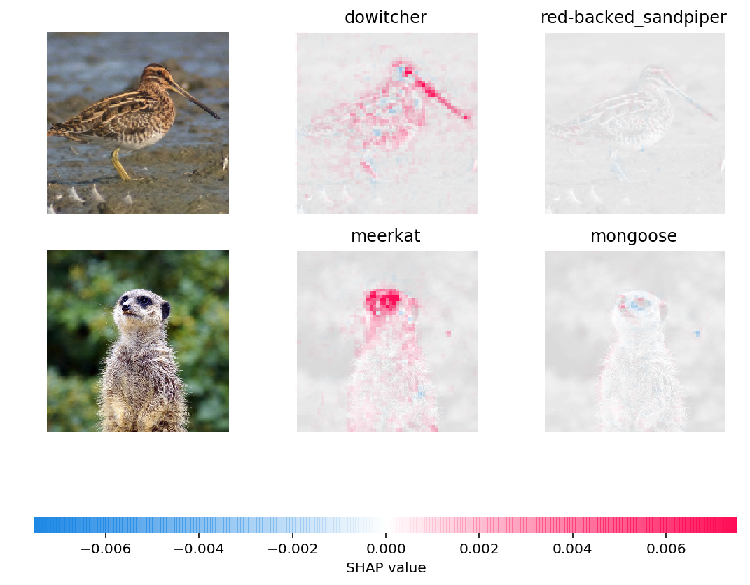
각 Class 를 예측함에 있어서, 어떤 부분이 중요한 역할을 했는지 볼 수 있습니다.
Reference
- XAI, 설명 가능한 인공지능, 인공지능을 해부하다 (안재현. 2020)
- 고려대학교 DMQA Seminar : An Overview of Model-Agnostic Interpretation Methods
- Interpretable Machine Learning : A Guide for Making Black Box Models Explainable (Christoph Molnar. 2021)
Code & Papers
SHAP: https://github.com/slundberg/shap- SHAP documentation : https://shap.readthedocs.io/en/latest/index.html
- Scott Lundberg et al. (2017). A Unified Approach to Interpreting Model Predictions
- Scott Lundberg et al. (2018). Consistent Individualized Feature Attribution for Tree Ensembles
- 허재혁님 Review : SHAP에 대한 모든 것
- daehani님 Review : Shapley value, SHAP, Tree SHAP

One night, I found myself in the midst of an online blackjack session that seemed to be going downhill fast. My initial enthusiasm quickly turned to frustration as my balance dwindled from $200 to just $20. I considered calling it a night, but https://montecrypto-casino-france.com a part of me was determined to turn things around. I decided to stay, focusing intently on each hand and sticking to basic strategy. Slowly but surely, my luck began to change. Small wins accumulated, and my balance started to rise. The excitement built as I clawed my way back up, eventually reaching a surprising $1,000. The sense of accomplishment and relief was immense. It was a powerful reminder of how persistence and strategy can turn a seemingly hopeless situation into a victory.