
ViT 코드리뷰
Vistion Transformer은 An Image is Worth 16x16 Words: Transformers for Image Recognition at Scale
으로 구글에서 2020년 10월 20일날 발표된 논문이다 이미지 분류에 Transformer을 사용하면서 SOTA를 달성했던 논문이다.
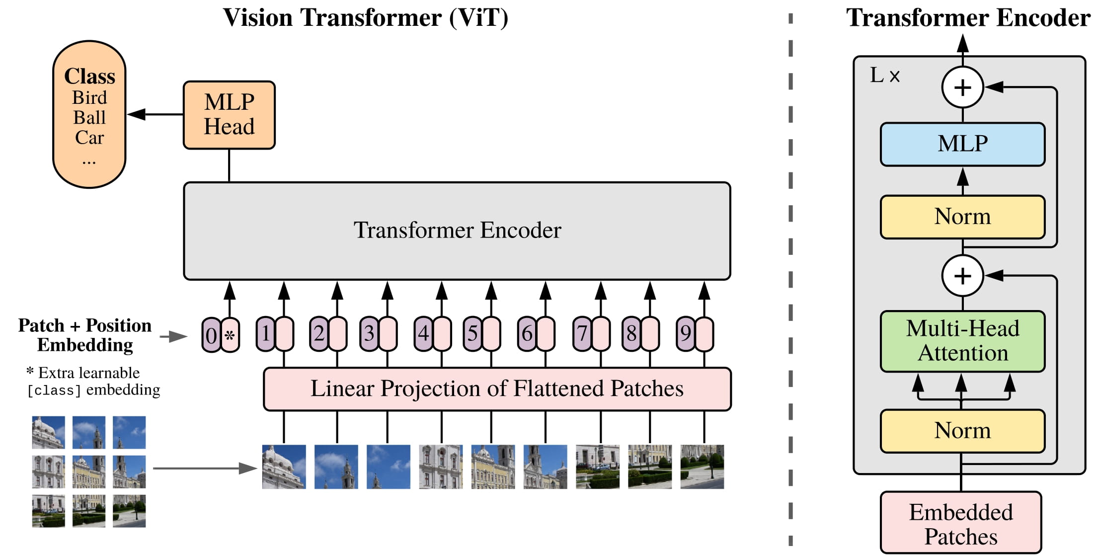
GIF를 살펴보면 이미지를 패치 사이즈로 자른 후에 이를 Linear Projection 시키고 Flatten시킨다. 이후 embedding을 한후 Transformer Encoder를 통과시킨다. 이를 MLP_head를 거쳐 최종적인 Classification을 수행한다.
1. 이미지를 패치 사이즈로 자른다.
2. 패치를 Linear Projection으로 Flatten 시킨다.
2-2. 각 Flatten시킨 패치를 Embedding 시킨다.
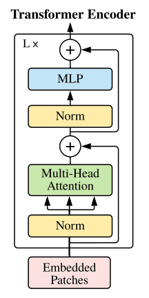
3. Transformer Encoder를 통과시킨다.
3-2 최종 Encoder Block
4. MLP Head를 거쳐 최종적인 Classification을 수행한다.
5. 최종 모델
1. 이미지를 패치 사이즈로 자른다. && 2. 각 Flatten시킨 패치를 Embedding 시킨다.
class image_embedding(nn.Module):
    def __init__(self,in_channels=3,img_size=224,patch_size=16,emb_dim = 16*16*3):
        super().__init__()

        self.rearrange = Rearrange('b c (num_w p1)(num_h p2) -> b (num_w num_h)(p1 p2 c)',p1=patch_size,p2=patch_size)
        #8 3 224 224 -> (8, 3, 224/16, 224/16) -> (8,14*14,16*16*3)
        self.linear = nn.Linear(in_channels*patch_size*patch_size,emb_dim)

        self.cls_token = nn.Parameter(torch.randn(1,1,emb_dim))

        n_patchs = img_size * img_size // patch_size**2
        self.positions = nn.Parameter(torch.randn(n_patchs + 1,emb_dim))

    def forward(self,x):
        batch,channel,width,height = x.shape
        #print('befor rearrange x shape:',x.shape)
        x = self.rearrange(x)
        #print('after rearrange x shape:',x.shape)
        x = self.linear(x)
        #print('cls_token shape:',self.cls_token.shape)
        c = repeat(self.cls_token,'() n d -> b n d',b = batch)
        x = torch.cat((c,x),1)
        #print('add cls_token shape:',x.shape)
        #print('positions shape:',self.positions.shape)
        x = torch.add(x,self.positions)
        print('last shape:',x.shape)

        return x
1. Rearrange 함수를 통해 8 3 224 224 -> (8, 3, 224/16, 224/16) -> (8,14x14,16x16x3) 으로 변형시킨다 그러면 이떄 (8,196,768)은 각 패치 196개의 대해 픽셀값이 768의 차원에 들어있다 이때 Color image이므로 16x16x3의 차원이 만들어지는 것이다.
2-1. self.linear 를 통해 각 768 차원을 Embedding 시키고 이후 Class token을 붙혀서 (8,196,768)의 차원을 (8,197,768)차원으로 만들어준다. 이때 Class Token은 nn.Parameter로 (1,1,768)로 만들어 학습 가능하게끔 만들어주게 되고 이는 최종적으로 마지막에 Classification을 수행하게 된다.
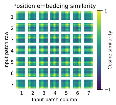
2-2. 이후 Positional Encoding 차원을 만들어주게 되는대 Positional Encoding 차원은 (8,197,768)을 nn.Parameter로 학습 가능하게끔 만들고 이를 더해준다. 이때 Positional Encoding은 아래와 같이 학습되어 각 패치의 위치를 학습하게 되는 부분이다.
3. Transformer Encoder를 통과시킨다.
class multi_head_attention(nn.Module):
    def __init__(self,emb_dim:int = 16*16*3,num_heads:int = 8,dropout_ratio:float=0.2,verbose=False,**kwargs):
        super(multi_head_attention,self).__init__()

        self.v = verbose
        self.emb_dim = emb_dim
        self.num_heads = num_heads
        self.scaling = (self.emb_dim // num_heads) ** (-0.5)

        self.value = nn.Linear(emb_dim,emb_dim)
        self.key = nn.Linear(emb_dim,emb_dim)
        self.query = nn.Linear(emb_dim,emb_dim)
        self.att_drop = nn.Dropout(dropout_ratio)

        self.linear = nn.Linear(emb_dim,emb_dim)

    def forward(self,x : Tensor) -> Tensor:

        Q = self.query(x)
        K = self.key(x)
        V = self.value(x)

        if self.v : print(Q.size(),K.size(),V.size())
        #q=k=v=patch_size *2 +1 & h * d  = emb_dim
        Q = rearrange(Q, 'b q (h d) -> b h q d',h = self.num_heads)
        K = rearrange(K, 'b k (h d) -> b h d k',h = self.num_heads)
        V = rearrange(V, 'b v (h d) -> b h v d',h = self.num_heads)
        if self.v : print(Q.size(),K.size(),V.size())

        weight = torch.matmul(Q,K)
        weight = weight * self.scaling
        if self.v: print(weight.size())

        attention = torch.softmax(weight, dim = -1)
        attention = self.att_drop(attention)
        if self.v: print(attention.size())

        context = torch.matmul(attention,V)
        context = rearrange(context,'b h q d -> b q (h d)')
        if self.v: print(context.size())

        x = self.linear(context)
        return x, attention
class mlp_block(nn.Module):
def __init__(self,emb_dim:int=16*16*3,forward_dim:int=4,dropout_ratio:float=0.2,**kwargs):
super(mlp_block,self).__init__()
self.linear_1 = nn.Linear(emb_dim,forward_dim * emb_dim)
self.dropout = nn.Dropout(dropout_ratio)
self.linear_2 = nn.Linear(emb_dim * forward_dim, emb_dim)
def forward(self,x):
x = self.linear_1(x)
x = nn.ReLU()(x)
x = self.dropout(x)
x = self.linear_2(x)
return x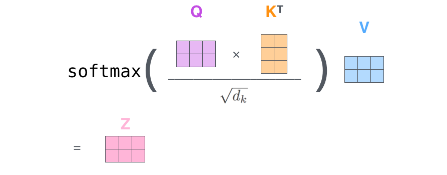
3-1. (8,197,768)의 차원을 각각 Q,K,V로 Linear층을 통과하여 각 토큰의 대한 표현이 Q,K,V로 투영된다.
Q = (8,197,768) ->(8,197,768)
K = (8,197,768) ->(8,197,768)
V = (8,197,768) ->(8,197,768)
3-2. 이 투영된 벡터에서 Multi-head attention을 통하여 각 토큰의 대한 768의 차원이 head의 갯수만큼 쪼개지게 된다 이때 위 코드에서 head는 8개이므로 실제 차원은
Q = (8,197,768) ->(8,8,197,96)
K = (8,197,768) ->(8,8,96,197)
V = (8,197,768) ->(8,8,197,96)
으로 쪼개지게 되는데 이를 보면 모든 토큰에 대해 emb_dim을 쪼개서 self-attention을 진행하겠다는 것이다.
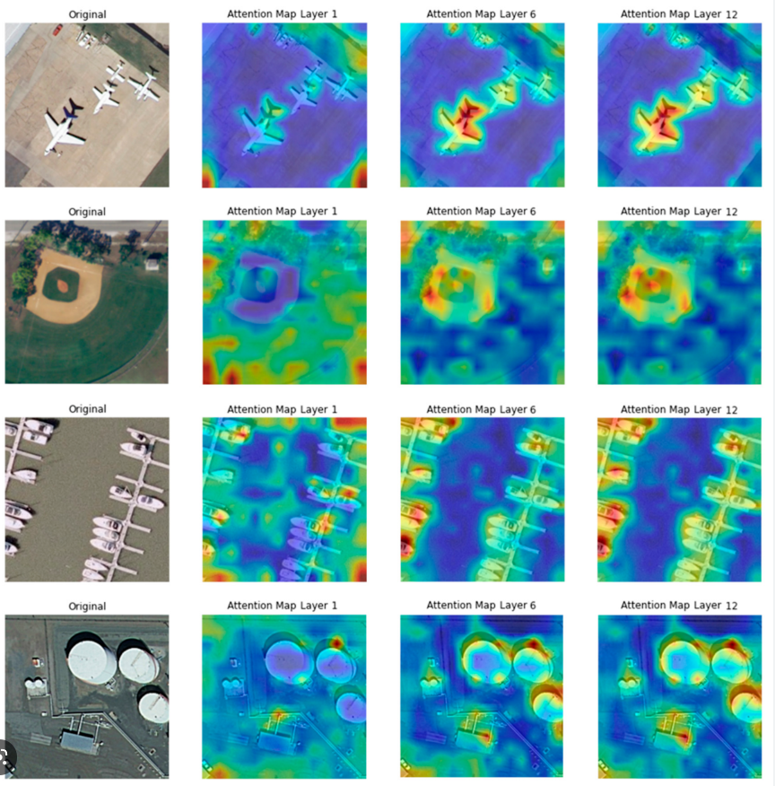
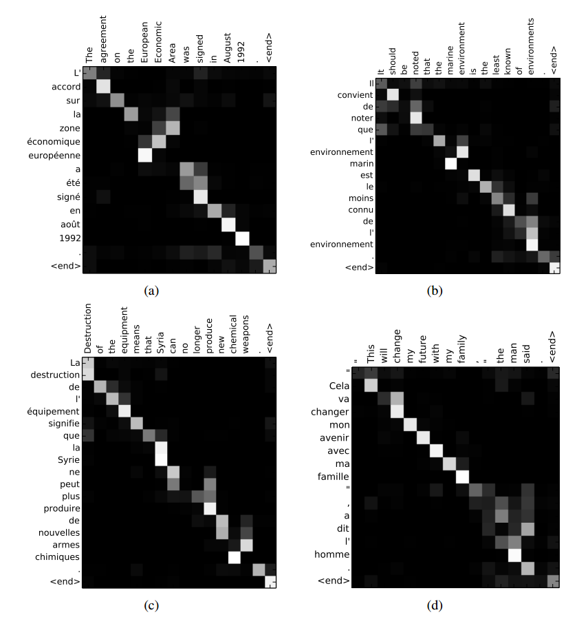
3-3. 이후 위의 수식을 통하여 각 head 8개의 대하여 attention을 구하게 되는데 이는 각 토큰과의 관계성을 보게되는 map이 나오게 된다.
아래 사진은 각각 Image와 단어에 대한 attention map을 시각화 한것이다.
즉 토큰과 토큰과의 관계성, 패치와 패치끼리의 관계성을 보는 것이다. 그러면 이를 softmax함수를 통과 하였으니 각 패치마다의 관계성 확률분포 라고 볼 수있다.
추후 V를 weight sum하게 되는데 V라는 투영된 이미지 값에
이러한 관계성 확률분포를 가하는 것이라고 볼 수 있다.
3-4. 그러면 우리는 헤드를 8개로 지정하였으니 8개의 attention map을 가지고 8개로 쪼개진 V에다가 각각 연산을 가하게 되는 이를 다시 합쳐준다. 어텐션 맵과 V를 matmul을 한 차원은 (8,8,197,96)이 되고 이를 다시 head와 emb_dim을 합쳐 준다. (8,8,197,96)->(8,197,768) 그럼 이때 단순히 차원을 조정하는 과정은 8개의 emb_dim에 대하여 단순히 붙여주게 됨으로 emb_dim간의 관계가 고려되지 않아 Linear층을 통과시킴으로써 다시 단순히 붙힌 연산을 섞어주게되고 emb_dim간의 관계를 보는것이라고 생각 할수 있다. 이후 최종적으로 Linear층을 통과한 벡터를 return 시켜준다.
3-5. 그럼 실제로 학습이 일어나는 부분은 attention map을 잘 만들기(모델링) 위해 Q,K,V가를 벡터로 투영될때 주요 학습이 일어난다고 보면된다.
3-5. 위 코드의 mlp_block은 mulit-head attention의 최종 아웃풋 값을 단순히 MLP를 통과 시켜 최종적으로 값을 재정렬하는 과정이라고 볼 수 있다. 이때 MLP를 통과하더라도 차원은 똑같이 유지된다.
3-2 최종 Encoder Block

class encoder_block(nn.Module):
    def __init__(self,emb_dim:int=16*16*3,num_heads:int=8,forward_dim:int=4,dropout_ratio:float=0.2):
        super(encoder_block,self).__init__()

        self.norm_1 = nn.LayerNorm(emb_dim)
        self.norm_1_G = nn.GELU()
        self.mha = multi_head_attention(emb_dim,num_heads,dropout_ratio)

        self.norm_2 = nn.LayerNorm(emb_dim)
        self.norm_2_G = nn.GELU()
        self.mlp = mlp_block(emb_dim,forward_dim,dropout_ratio)
        self.residual_dropout = nn.Dropout(dropout_ratio)

    def forward(self,x):
        x2 = self.norm_1(x)
        x2 = self.norm_1_G(x)
        x2 , attention = self.mha(x2)
        x = torch.add(x2,x)

        x2 = self.norm_2(x)
        x2 = self.norm_2_G(x)
        x2 = self.mlp(x2)
        x = torch.add(x2,x)

        return x,attention
1. 실제 Encoder Block은 처음 입력으로 들어온 (8,197,768) 이떄 이 차원은 QKV를 아직 만들지 않은 차원이다. LayerNorm과 GELU를 통과시키고 mulit_head_attention을 수행한다. 이떄 최종적인 output값과 처음 input의 차원은 동일 하길때문에 이를 단순히 add 해준다. 그후 Layernorm과 GELU를 통과시키고 MLP를 거친다. 추후에 처음 mulit-head attention을 거친 output과
마지막 MLP를 통과한 output을 add 해주어 최종적인(8,197,768)의 차원을 만든다. 이로써 ViT encoder_block은 input과 output이 동일하다.
4. MLP Head를 거쳐 최종적인 Classification을 수행한다.
class vision_transformer(nn.Module):
    def __init__(self,in_channels:int=3,img_size:int=224,patch_size:int=16,emb_dim:int=16*16*3,
                n_enc_layers:int=15,num_heads:int=3,forward_dim:int=4,dropout_ratio:float=0.2,n_classes:int=1000):
        super(vision_transformer,self).__init__()

        self.image_embedding = image_embedding(in_channels,img_size,patch_size,emb_dim)
        encoder_module = [encoder_block(emb_dim,num_heads,forward_dim,dropout_ratio)for _ in range(n_enc_layers)]
        self.encoder_module = nn.ModuleList(encoder_module)

        self.reduce_layer = Reduce('b n e -> b e',reduction='mean')
        self.normalization = nn.LayerNorm(emb_dim)
        self.classification_head = nn.Linear(emb_dim,n_classes)

    def forward(self,x):
        x = self.image_embedding(x)
        attentions = [block(x)[1] for block in self.encoder_module]
        #print('before reduce x size : ',x)
        x = self.reduce_layer(x)#(8 768)
        x = self.normalization(x)#(8 768)
        #print(x.shape)
        x = self.classification_head(x)(8,1000)

        return x
코드를 보게되면 이미지에 대해 embedding을 진행해주게 되고 우리가 만든 Encoder_block을 input과output의 차원이 동일하여 위 코드에서는 15개를 쌓게 된다. 추후 모든 Encoder_block을 최종적으로 통과한 벡터에 reduce_layer을 적용하게 되는데 원래는 우리가 처음에 만든 class_token만을 사용하여 (8,768)을 만들지만 큰 차이가 없음으로 모든 토큰에 대하여 mean을 취해주어 (8,768)을 만들어준다. 이후 이를 다시 Layer_norm시키고 마지막 classification_head을 통과하여 최종적인 Classification을 수행하게 된다.
5. 최종 모델
model = vision_transformer()
device = torch.device("cuda" if torch.cuda.is_available() else "cpu")
model.to(device)
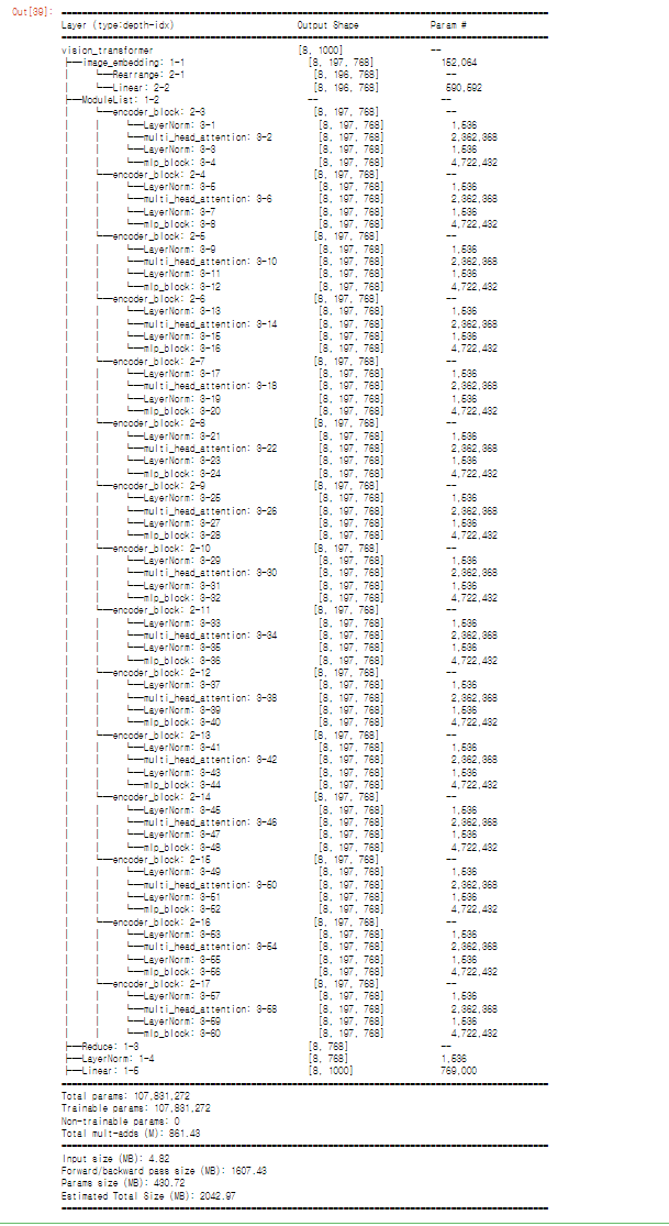
summary(model,(8,3, 224, 224))이와 같이 생겼으며 Linear층은 원래 파라미터 갯수가 많은데 Linear층을 많이 사용하는 Encoder block을 15개를 쌓아 약 1억개의 파라미터 수가 나오게 된다.
회고
vit는 기존에 논문리뷰도 진행하였고 다시 한번 코드를 본다는 마인드로 쓰게 되었다 심화과제에서 정태문 조교님께 질문한 답변이 큰 도움이 된것 같다. 그리고 귀여운 개발진스 한마리 물어가면 좋겠다.