스터디노트 (DeepLearning 8)

유방암예측

# 유방암 예측

import pandas as pd
import seaborn as sns
import matplotlib.pyplot as plt

import torch
import torch.nn as nn
import torch.nn.functional as F
import torch.optim as optim

from sklearn.datasets import load_breast_cancer
cancer = load_breast_cancer()

print(cancer.DESCR)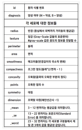

# 데이터 정리

df = pd.DataFrame(cancer.data, columns=cancer.feature_names)
df['class'] = cancer.target

df.tail()

# 관심있는 컬럼 정리

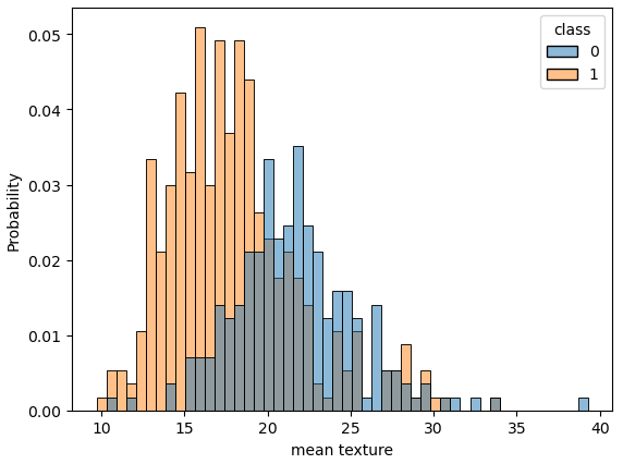
cols = ['mean radius', 'mean texture', 'mean smoothness', 'mean compactness',
        'mean concave points', 'worst radius', 'worst texture', 'worst smoothness',
        'worst compactness', 'worst concave points', 'class']

for c in cols[:-1]:
    sns.histplot(df, x=c, hue=cols[-1], bins=50, stat='probability')
    plt.show()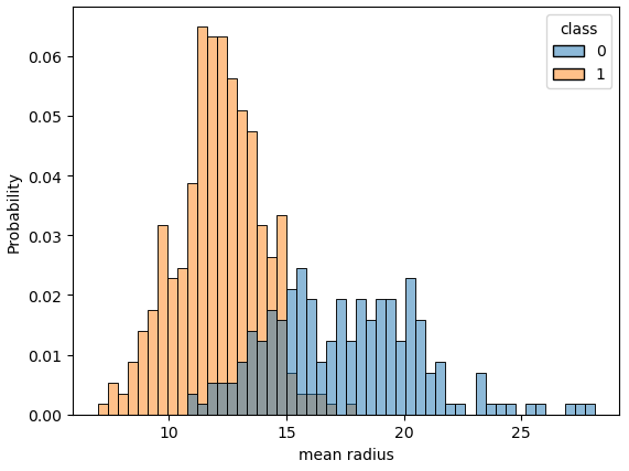

# torch import

data = torch.from_numpy(df[cols].values).float()
data.shape

# 데이터를 라벨과 특성으로 나누기
# Split x and y

x = data[:, :-1]
y = data[:, -1:]

print(x.shape, y.shape)

# 하이퍼파라미터 설정
# define confiurations

n_epochs = 200000
learning_rate = 1e-2
print_interval = 10000

# my model 작성

class MyModel(nn.Module):
    def __init__(self, input_dim, output_dim):
        self.input_dim = input_dim
        self.output_dim = output_dim
        
        super().__init__() # nn.Module 모듈의 속성 상속받을 수 있음
        
        self.linear = nn.Linear(input_dim, output_dim)
        self.act = nn.Sigmoid()
    
    def forward(self, x):
        y = self.act(self.linear(x))
        
        return y

# 모델 선언, loss, optim 선언

model = MyModel(input_dim=x.size(-1), output_dim=y.size(-1)) # size(-1) : 마지막 차원

crit_func = nn.BCELoss() 
# BCELoss함수를 쓸땐 마지막 레이어를 시그모이드함수를 적용시켜줘야 한다.
# https://wooono.tistory.com/387

optimizer = optim.SGD(model.parameters(), lr=learning_rate)

# 학습 시작

for i in range(n_epochs):
    y_hat = model(x)
    loss = crit_func(y_hat, y)
    
    optimizer.zero_grad()
    loss.backward()
    
    optimizer.step()
    
    if (i + 1) % print_interval == 0:
        print('Epoch %d : loss = %.4e' %(i+1, loss))

# acc 계산

correct_cnt = (y == (y_hat > 0.5)).sum()
total_cnt = float(y.size(0))

print('Accuracy : %.4f' %(correct_cnt / total_cnt))

# 예측값의 분포 확인

df = pd.DataFrame(torch.cat([y, y_hat], dim=1).detach().numpy(), columns=['y', 'y_hat'])
df

sns.histplot(df, x='y_hat', hue='y', bins=50, stat='probability')
# bins = : 막대그래프의 폭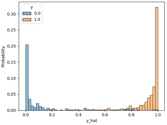

어렵다..ㅠㅠ
💻 출처 : 제로베이스 데이터 취업 스쿨