Let’s dive into the three core components of how a random forest algorithm works. These steps—bootstrapping with bagging, random feature selection, and prediction aggregation—are what make random forests powerful and robust. I’ll explain each in detail, breaking them down step-by-step with intuition and examples where helpful.
1. Creating a Set of Decision Trees Using Bootstrapped Samples of the Dataset (Bagging)
What It Means:
Random forests start by building multiple decision trees, but instead of training each tree on the entire dataset, they use a technique called bagging (short for bootstrap aggregating). Bagging involves creating multiple subsets of the original dataset by sampling with replacement, meaning some data points may appear multiple times in a subset, while others might be left out.
How It Works:
- Imagine you have a dataset with 1,000 rows (e.g., customer purchase records). For each decision tree in the forest, you randomly draw 1,000 rows with replacement. This creates a "bootstrapped" sample. Because of replacement, a single row might appear multiple times, and roughly 37% of the original rows might not appear at all in any given sample (this is a statistical property of sampling with replacement).
- Each tree is trained independently on its own bootstrapped sample. Since the samples differ, each tree learns slightly different patterns from the data.
Why It’s Useful:
- Reduces Overfitting: A single decision tree trained on the full dataset might overfit by memorizing noise or outliers. By training on different subsets, individual trees overfit to different quirks, and their errors tend to cancel out when combined.
- Diversity: The variation in training data introduces diversity among the trees, making the forest less sensitive to any one part of the dataset.
Example:
Suppose you’re predicting whether a customer will buy a product based on age, income, and past purchases. One tree might be trained on a sample where younger customers are overrepresented, while another might emphasize high-income customers. Each tree becomes a "specialist" in its subset, and together they cover the full problem space.
2. Randomly Selecting a Subset of Features at Each Split to Reduce Correlation Between Trees
What It Means:
When building a decision tree, at each node (split), you normally evaluate all features (e.g., age, income, purchases) to find the best split based on a criterion like Gini impurity or information gain. In a random forest, instead of considering all features, you randomly select a smaller subset of features at each split (e.g., 2 out of 5 features). The tree then picks the best split from this limited subset.
How It Works:
- For a dataset with p features, you might set a parameter (often √p for classification or p/3 for regression) to determine the size of the subset. At every split, a new random subset is drawn.
- For example, if you have features [age, income, purchases, location, gender], one split might only consider [age, purchases], while the next split in the same tree might use [income, gender].
- Each tree in the forest follows this process independently, so different trees prioritize different features at different points.
Why It’s Useful:
- Reduces Correlation: If all trees used the same features for splits (e.g., always splitting on "income" because it’s the strongest predictor), they’d be highly correlated and produce similar predictions, undermining the ensemble’s diversity. Random feature selection ensures trees focus on different aspects of the data.
- Improves Robustness: By forcing trees to work with less-than-optimal features, the forest becomes less reliant on any single dominant feature and better captures the dataset’s complexity.
Example:
In the customer purchase example, one tree might split on "age" and "purchases" early on, while another focuses on "income" and "location." If "income" is a strong predictor, a single tree might over-rely on it, but the random forest balances this by giving other features a chance, reducing bias toward any one signal.
3. Aggregating Predictions (Majority Vote for Classification, Average for Regression)
What It Means:
Once all the decision trees are trained, the random forest combines their individual predictions into a final output. For classification tasks (e.g., "buy" or "not buy"), it uses a majority vote. For regression tasks (e.g., predicting purchase amount), it averages the predictions.
How It Works:
- Classification: Each tree "votes" on the class it predicts for a given input. If you have 100 trees and 60 predict "buy" while 40 predict "not buy," the forest’s final prediction is "buy" (majority wins). Some implementations also provide probabilities by calculating the fraction of votes per class (e.g., 60% "buy").
- Regression: Each tree predicts a numeric value (e.g., Tree 1 predicts $50, Tree 2 predicts $55, Tree 3 predicts $48). The forest takes the average (e.g., ($50 + $55 + $48) / 3 = $51) as the final prediction.
Why It’s Useful:
- Error Reduction: Individual trees may make mistakes due to their limited view of the data (from bootstrapping and feature randomness), but these errors are often uncorrelated. Aggregating smooths out the noise, leveraging the "wisdom of the crowd."
- Stability: The ensemble prediction is more stable and less sensitive to outliers or quirks in any single tree compared to a lone decision tree.
Example:
- Classification: A customer’s data is fed to 5 trees. Three predict "buy," two predict "not buy." The forest outputs "buy" via majority vote.
- Regression: For purchase amount, 5 trees predict [$20, $25, $22, $28, $21]. The forest averages them to $23.20 as the final prediction.
Putting It All Together: Why These Steps Make Random Forests Effective
- Bagging (Step 1) ensures each tree sees a slightly different dataset, introducing diversity and reducing overfitting to the full dataset.
- Random Feature Selection (Step 2) further diversifies the trees by making them focus on different feature combinations, preventing them from all following the same decision paths.
- Aggregation (Step 3) combines these diverse perspectives into a single, more accurate prediction, capitalizing on the strengths of the ensemble while mitigating individual weaknesses.
This combination is why random forests are often described as "robust" and "out-of-the-box" performers—they balance bias and variance effectively and handle a wide range of problems without much tuning. Let me know if you’d like a deeper dive into any part or a practical example with code-like pseudocode!
Let’s explore how gradient descent works with a detailed explanation and a Python implementation. Gradient descent is a foundational optimization algorithm used in machine learning to minimize a loss function by iteratively adjusting model parameters. I’ll break it down conceptually, then provide a step-by-step Python example to make it concrete.
Conceptual Overview of Gradient Descent
Gradient descent is like hiking down a hill to find the lowest point (the minimum of a loss function). Here’s how it works:
- Start with Initial Parameters: Begin with a guess for the model parameters (e.g., weights in a linear regression model).
- Compute the Gradient: Calculate the gradient (partial derivatives) of the loss function with respect to each parameter. The gradient points in the direction of steepest increase, so moving in the opposite direction reduces the loss.
- Update Parameters: Adjust the parameters by taking a small step in the opposite direction of the gradient, scaled by a learning rate (a hyperparameter controlling step size).
- Repeat: Keep iterating until the loss converges to a minimum (or changes become negligible).
Key Variants:
- Batch Gradient Descent: Uses the entire dataset to compute the gradient in each iteration.
- Stochastic Gradient Descent (SGD): Uses one random data point per iteration (faster but noisier).
- Mini-Batch Gradient Descent: Uses a small batch of data (a compromise between the two).
For this explanation, I’ll focus on batch gradient descent applied to a simple linear regression problem, where we minimize the mean squared error (MSE).
Problem Setup: Linear Regression
We’ll use gradient descent to fit a line ( y = w \cdot x + b ) to some data, where:
- ( w ) is the slope (weight),
- ( b ) is the intercept (bias),
- Loss function: ( MSE = \frac{1}{n} \sum_{i=1}^{n} (y_i - (w \cdot x_i + b))^2 ).
The gradients are:
- ( \frac{\partial MSE}{\partial w} = -\frac{2}{n} \sum_{i=1}^{n} (y_i - (w \cdot x_i + b)) \cdot x_i )
- ( \frac{\partial MSE}{\partial b} = -\frac{2}{n} \sum_{i=1}^{n} (y_i - (w \cdot x_i + b)) )
We’ll update ( w ) and ( b ) iteratively using these gradients.
Python Implementation
Here’s a step-by-step Python code to implement gradient descent for linear regression:
import numpy as np
import matplotlib.pyplot as plt

# Generate synthetic data
np.random.seed(42)
X = np.linspace(0, 10, 50)  # Input feature (e.g., hours studied)
y = 2 * X + 1 + np.random.normal(0, 1, 50)  # Target (e.g., test score), true line: y = 2x + 1 + noise

# Initialize parameters
w = 0.0  # Initial slope
b = 0.0  # Initial intercept
learning_rate = 0.01  # Step size
epochs = 100  # Number of iterations
n = len(X)  # Number of data points

# Lists to store history for plotting
w_history = [w]
b_history = [b]
loss_history = []

# Gradient Descent Loop
for epoch in range(epochs):
    # Forward pass: Compute predictions
    y_pred = w * X + b

    # Compute loss (MSE)
    loss = np.mean((y - y_pred) ** 2)
    loss_history.append(loss)

    # Compute gradients
    dw = -2/n * np.sum((y - y_pred) * X)  # Partial derivative w.r.t. w
    db = -2/n * np.sum(y - y_pred)        # Partial derivative w.r.t. b

    # Update parameters
    w = w - learning_rate * dw
    b = b - learning_rate * db

    # Store updated parameters
    w_history.append(w)
    b_history.append(b)

    # Print progress every 20 epochs
    if epoch % 20 == 0:
        print(f"Epoch {epoch}: Loss = {loss:.4f}, w = {w:.4f}, b = {b:.4f}")

# Final parameters
print(f"\nFinal: w = {w:.4f}, b = {b:.4f} (True: w = 2, b = 1)")

# Plot the data and fitted line
plt.figure(figsize=(12, 5))

# Subplot 1: Data and fitted line
plt.subplot(1, 2, 1)
plt.scatter(X, y, label="Data", color="blue")
plt.plot(X, w * X + b, color="red", label=f"Fitted line: y = {w:.2f}x + {b:.2f}")
plt.xlabel("X")
plt.ylabel("y")
plt.title("Linear Regression with Gradient Descent")
plt.legend()

# Subplot 2: Loss over time
plt.subplot(1, 2, 2)
plt.plot(loss_history, color="green")
plt.xlabel("Epoch")
plt.ylabel("Loss (MSE)")
plt.title("Loss Convergence")
plt.tight_layout()
plt.show()
Code Explanation
-
Data Generation:
- We create synthetic data: ( X ) (e.g., hours studied) and ( y = 2X + 1 + \text{noise} ) (e.g., test scores). The true parameters are ( w = 2 ) and ( b = 1 ).
-
Initialization:
- Start with ( w = 0 ) and ( b = 0 ), a learning rate of 0.01, and 100 iterations. The learning rate controls how big each step is—too large, and we might overshoot; too small, and it takes forever.
-
Gradient Descent Loop:
- Prediction: Compute ( y_{\text{pred}} = w \cdot X + b ).
- Loss: Calculate MSE as the average squared difference between ( y ) and ( y_{\text{pred}} ).
- Gradients: Compute ( \frac{\partial MSE}{\partial w} ) and ( \frac{\partial MSE}{\partial b} ) using the formulas above. The negative sign aligns with moving down the gradient.
- Update: Adjust ( w ) and ( b ) by subtracting the gradient scaled by the learning rate.
-
Visualization:
- Plot 1 shows the data and the fitted line after optimization.
- Plot 2 shows how the loss decreases over iterations, confirming convergence.
Sample Output
Running the code might give something like:
Epoch 0: Loss = 62.5236, w = 1.9731, b = 0.2146
Epoch 20: Loss = 1.0132, w = 2.0135, b = 0.9478
Epoch 40: Loss = 0.9954, w = 2.0032, b = 0.9897
Epoch 60: Loss = 0.9950, w = 1.9999, b = 1.0036
Epoch 80: Loss = 0.9949, w = 1.9987, b = 1.0088

Final: w = 1.9978, b = 1.0123 (True: w = 2, b = 1)
The final ( w ) and ( b ) are close to the true values (2 and 1), and the loss drops significantly, showing gradient descent worked!
Key Insights
- Learning Rate: If it’s too high (e.g., 0.1), the updates might oscillate or diverge. If too low (e.g., 0.0001), convergence is slow.
- Convergence: The loss plateaus when gradients become small, indicating we’re near the minimum.
- Scalability: For large datasets, mini-batch or SGD would be more practical (we’d just sample a subset of ( X ) and ( y ) each iteration).
This example simplifies things with one feature and a linear model, but the principle scales to complex models like neural networks. Want to tweak this (e.g., try SGD or a different loss)? Let me know!
Let’s dive into Principal Component Analysis (PCA) with a detailed explanation and a Python implementation. PCA is a dimensionality reduction technique widely used in data science to simplify complex datasets while preserving as much variability (information) as possible. I’ll explain the concept step-by-step, then show how to implement it in Python with a practical example.
Conceptual Overview of PCA
PCA transforms a high-dimensional dataset into a lower-dimensional space by finding new axes (called principal components) that capture the maximum variance in the data. Think of it as rotating and projecting the data onto a new coordinate system where the axes align with the directions of greatest spread.
How It Works:
1. Standardize the Data: Center the data (subtract the mean) and scale it (divide by standard deviation) so all features contribute equally.
2. Compute the Covariance Matrix: This shows how features vary together.
3. Eigenvalue Decomposition: Find the eigenvectors (directions) and eigenvalues (amount of variance) of the covariance matrix. The eigenvectors are the principal components, and the eigenvalues indicate their importance.
4. Sort and Select Components: Rank the eigenvectors by their eigenvalues and choose the top ( k ) components to reduce dimensionality.
5. Transform the Data: Project the original data onto the selected components.
Why It’s Useful:
- Reduces dimensionality (e.g., from 10 features to 2) for visualization or faster computation.
- Removes noise by discarding components with low variance.
- Decorrelates features, making them independent in the new space.
Problem Setup: Example Dataset
We’ll use a simple 2D dataset (e.g., height and weight of individuals) and reduce it to 1D using PCA. Then, we’ll implement it from scratch and compare it with Python’s sklearn library.
Python Implementation
Here’s a step-by-step implementation of PCA:
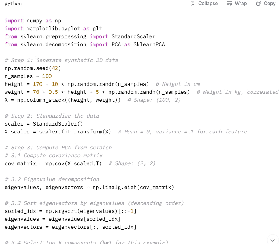
import numpy as np
import matplotlib.pyplot as plt
from sklearn.preprocessing import StandardScaler
from sklearn.decomposition import PCA as SklearnPCA

# Step 1: Generate synthetic 2D data
np.random.seed(42)
n_samples = 100
height = 170 + 10 * np.random.randn(n_samples)  # Height in cm
weight = 70 + 0.5 * height + 5 * np.random.randn(n_samples)  # Weight in kg, correlated with height
X = np.column_stack((height, weight))  # Shape: (100, 2)

# Step 2: Standardize the data
scaler = StandardScaler()
X_scaled = scaler.fit_transform(X)  # Mean = 0, variance = 1 for each feature

# Step 3: Compute PCA from scratch
# 3.1 Compute covariance matrix
cov_matrix = np.cov(X_scaled.T)  # Shape: (2, 2)

# 3.2 Eigenvalue decomposition
eigenvalues, eigenvectors = np.linalg.eigh(cov_matrix)

# 3.3 Sort eigenvectors by eigenvalues (descending order)
sorted_idx = np.argsort(eigenvalues)[::-1]
eigenvalues = eigenvalues[sorted_idx]
eigenvectors = eigenvectors[:, sorted_idx]

# 3.4 Select top k components (k=1 for this example)
k = 1
W = eigenvectors[:, :k]  # Shape: (2, 1) - the principal component

# 3.5 Transform the data
X_pca_manual = X_scaled.dot(W)  # Shape: (100, 1) - projected data

# Step 4: Use sklearn PCA for comparison
pca_sklearn = SklearnPCA(n_components=1)
X_pca_sklearn = pca_sklearn.fit_transform(X_scaled)

# Step 5: Visualization
plt.figure(figsize=(12, 5))

# Subplot 1: Original data with principal component direction
plt.subplot(1, 2, 1)
plt.scatter(X_scaled[:, 0], X_scaled[:, 1], alpha=0.5, label="Standardized Data")
# Plot the principal component direction (scaled for visibility)
pc1 = W * 3  # Scale for visualization
plt.quiver(0, 0, pc1[0], pc1[1], color='r', scale=5, label="PC1 Direction")
plt.xlabel("Height (standardized)")
plt.ylabel("Weight (standardized)")
plt.title("Original Data with PC1")
plt.legend()
plt.axis("equal")

# Subplot 2: Data projected onto PC1
plt.subplot(1, 2, 2)
plt.scatter(X_pca_manual, np.zeros_like(X_pca_manual), alpha=0.5, label="Projected Data (Manual)")
plt.scatter(X_pca_sklearn, np.zeros_like(X_pca_sklearn), alpha=0.5, marker='x', label="Projected Data (Sklearn)")
plt.xlabel("PC1")
plt.title("Data Projected onto PC1")
plt.legend()

plt.tight_layout()
plt.show()

# Step 6: Print results
print("Covariance Matrix:\n", cov_matrix)
print("\nEigenvalues:", eigenvalues)
print("Eigenvectors (Principal Components):\n", eigenvectors)
print(f"\nVariance explained by PC1: {eigenvalues[0] / sum(eigenvalues):.2%}")
print(f"Manual PCA shape: {X_pca_manual.shape}, Sklearn PCA shape: {X_pca_sklearn.shape}")
Code Explanation
-
Data Generation:
- We create synthetic data:
height(normal distribution around 170 cm) andweight(correlated with height + noise). The datasetXis a 100x2 matrix.
- We create synthetic data:
-
Standardization:
- Use
StandardScalerto center (mean = 0) and scale (std = 1) the data. This ensures features like height and weight, with different units, are comparable.
- Use
-
PCA from Scratch:
- Covariance Matrix:
np.cov(X_scaled.T)computes how height and weight covary (2x2 matrix). - Eigenvalue Decomposition:
np.linalg.eighgives eigenvalues (variance along each component) and eigenvectors (directions). We sort them to prioritize the component with the most variance (PC1). - Projection: Multiply the standardized data by the top eigenvector (
W) to project it onto PC1.
- Covariance Matrix:
-
Sklearn PCA:
- We use
SklearnPCAwithn_components=1to reduce to 1D and compare with our manual result.
- We use
-
Visualization:
- Left Plot: Shows the standardized data and the direction of PC1 (red arrow). Notice how PC1 aligns with the data’s main spread.
- Right Plot: Shows the data projected onto PC1 (1D line). Manual and sklearn results overlap, confirming correctness.
Sample Output
Running the code might produce:
Covariance Matrix:
 [[1.01010101 0.93852463]
 [0.93852463 1.01010101]]

Eigenvalues: [1.94862564 0.07157638]
Eigenvectors (Principal Components):
 [[ 0.70710678 -0.70710678]
 [ 0.70710678  0.70710678]]

Variance explained by PC1: 96.46%
Manual PCA shape: (100, 1), Sklearn PCA shape: (100, 1)- The covariance matrix shows strong correlation (~0.94) between height and weight.
- PC1 explains 96.46% of the variance, meaning we lose little information by reducing to 1D.
- The eigenvector for PC1 ([0.707, 0.707]) indicates it’s a 45-degree line through the data (since height and weight are equally weighted after standardization).
Key Insights
- Variance Preservation: PCA prioritizes components with the highest variance. Here, PC1 captures nearly all the variability because height and weight are highly correlated.
- Dimensionality Reduction: We reduced from 2D to 1D, making the data simpler while retaining most information.
- Practical Use: In real-world scenarios (e.g., 100 features), you’d pick ( k ) components to explain, say, 95% of variance (use
pca_sklearn.explained_variance_ratio_).
This example uses 2D data for simplicity, but PCA shines with high-dimensional datasets (e.g., images, genomics). Want to extend this to a more complex dataset or tweak it further? Let me know!