Algorithm

📌 CLRS 공부 플랜

목표: 6개월 동안 CLRS(Introduction to Algorithms, 4th Edition)를 학습하며, 알고리즘 설계 및 분석 역량을 강화하기.

1️⃣ 학습 방법

• 이론 학습: 매주 특정 장을 정해 읽고 개념 정리
• 코딩 연습: 해당 장의 알고리즘을 Python으로 구현
• 문제 풀이: 연습문제 및 LeetCode, Codeforces 활용
• 리뷰 및 복습: 2~3주마다 한 번씩 개념 복습

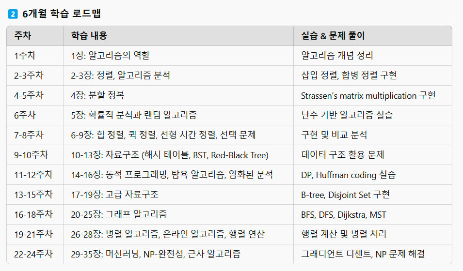
2️⃣ 6개월 학습 로드맵

주차	학습 내용	실습 & 문제 풀이
1주차	1장: 알고리즘의 역할	알고리즘 개념 정리
2-3주차	2-3장: 정렬, 알고리즘 분석	삽입 정렬, 합병 정렬 구현
4-5주차	4장: 분할 정복	Strassen’s matrix multiplication 구현
6주차	5장: 확률적 분석과 랜덤 알고리즘	난수 기반 알고리즘 실습
7-8주차	6-9장: 힙 정렬, 퀵 정렬, 선형 시간 정렬, 선택 문제	구현 및 비교 분석
9-10주차	10-13장: 자료구조 (해시 테이블, BST, Red-Black Tree)	데이터 구조 활용 문제
11-12주차	14-16장: 동적 프로그래밍, 탐욕 알고리즘, 암화된 분석	DP, Huffman coding 실습
13-15주차	17-19장: 고급 자료구조	B-tree, Disjoint Set 구현
16-18주차	20-25장: 그래프 알고리즘	BFS, DFS, Dijkstra, MST
19-21주차	26-28장: 병렬 알고리즘, 온라인 알고리즘, 행렬 연산	행렬 계산 및 병렬 처리
22-24주차	29-35장: 머신러닝, NP-완전성, 근사 알고리즘	그래디언트 디센트, NP 문제 해결

---

📌 1장 요약: 알고리즘의 역할

1. 알고리즘이란?

   • 특정 입력을 받아 정해진 연산을 수행하여 결과를 출력하는 명확한 절차.
   • 예: 정렬 알고리즘, 최단 경로 알고리즘.

2. 알고리즘이 중요한 이유

   • 효율성: 같은 문제를 풀더라도 알고리즘에 따라 속도가 다름.
   • 자원 절약: 계산 속도, 메모리 사용량 최적화.
   • 기술 발전: 컴퓨터가 빠르더라도, 비효율적인 알고리즘은 성능 저하를 초래함.

3. 알고리즘과 기술 발전

   • 하드웨어가 발전해도 비효율적인 알고리즘을 쓰면 성능이 제한됨.
   • 예제: 삽입 정렬(O(n²)) vs 병합 정렬(O(n log n))

4. 알고리즘의 실제 응용

   • 검색 엔진(Google) → 페이지 랭킹 알고리즘
   • 유전자 분석 → 동적 프로그래밍 기반 서열 정렬
   • 네트워크 경로 탐색 → 다익스트라 알고리즘

5. 알고리즘의 난제

   • NP-완전 문제: 빠른 해결책이 없는 문제 (예: 외판원 문제)
   • 머신러닝의 대두 → 알고리즘 설계와 결합하여 최적화

🔥 다음 단계: 2장(삽입 정렬, 알고리즘 분석) 공부 시작! 🚀
이 플랜이나 요약에서 수정하거나 보완하고 싶은 부분이 있으면 말해줘!

Gyver Tc, [2/17/2025 1:24 PM]

📌 2-3주차 내용 정리 (CLRS 4판, 2-3장)

🔹 2장: 삽입 정렬 (Insertion Sort)

1. 삽입 정렬 개념

   • 배열을 정렬할 때 앞쪽부터 하나씩 정렬된 상태로 유지하며, 새로운 원소를 적절한 위치에 삽입하는 방식
   • 직관적으로 사람들이 숫자를 정렬하는 방식과 유사
   • 시간 복잡도: O(n²) (최악), O(n) (최선, 이미 정렬된 경우)

2. 삽입 정렬 알고리즘 (의사코드)
   def insertion_sort(arr):
   for i in range(1, len(arr)):
   key = arr[i]
   j = i - 1
   while j >= 0 and arr[j] > key:
   arr[j + 1] = arr[j]
   j -= 1
   arr[j + 1] = key

3. 삽입 정렬 분석
   • 최선: 이미 정렬된 경우, 비교만 수행 → O(n)
   • 최악: 역순 정렬된 경우, 모든 원소를 이동해야 함 → O(n²)
   • 작은 데이터셋에서 효율적, 하지만 큰 데이터셋에서는 비효율적

---

🔹 3장: 알고리즘 분석 (Analyzing Algorithms)

1. 입력 크기 (Input Size)

   • 알고리즘의 수행 시간을 측정할 때 입력 크기(n) 을 기준으로 분석
   • 정렬의 경우, 배열의 길이(n)

2. 점근 표기법 (Asymptotic Notation)

   • O(빅오, Big-O): 최악의 경우 수행 시간 상한
   • Ω(오메가, Omega): 최상의 경우 수행 시간 하한
   • Θ(세타, Theta): 평균적으로 수행 시간이 일정한 경우

3. 재귀적 알고리즘 분석

   • 마스터 정리(Master Theorem): 분할 정복 알고리즘의 수행 시간 계산
   • 예: 병합 정렬 (Merge Sort) → O(n log n)

4. 실전 활용

   • 작은 데이터셋 → 삽입 정렬 (O(n²) 허용 가능)
   • 큰 데이터셋 → 병합 정렬, 퀵 정렬 등 (O(n log n)) 사용

---

📌 2-3주차 학습 실습

✅ [실습1] 삽입 정렬 구현 및 실행 시간 비교
✅ [실습2] 빅오 분석 연습 (O, Ω, Θ 표기 연습)
✅ [실습3] 마스터 정리 적용하여 분할 정복 알고리즘 분석

이제 4장(분할 정복)으로 넘어가면 좀 더 효율적인 알고리즘을 다룰 수 있어!
이해 안 되는 부분이나 추가 질문 있으면 알려줘 🚀

Gyver Tc, [2/17/2025 1:26 PM]

📌 4-5주차 내용 정리 (CLRS 4판, 4-5장)

목표: 분할 정복 기법을 이해하고, 효율적인 알고리즘 구현 능력을 키우기

---

🔹 4장: 분할 정복 (Divide and Conquer)

1. 개념

• 문제를 작은 하위 문제로 나누고, 각각을 해결한 후 병합하는 방식
• 재귀적으로 적용되며, 시간 복잡도를 줄이는 핵심 기법

2. 일반적인 구조 (Divide, Conquer, Combine)

• Divide: 문제를 작은 부분으로 나눈다.
• Conquer: 각 부분을 재귀적으로 해결한다.
• Combine: 부분 결과를 합쳐 최종 해를 구한다.

3. 분할 정복 알고리즘 예시

• 병합 정렬 (Merge Sort): O(n log n)
• 퀵 정렬 (Quick Sort): O(n log n) (최악 O(n²))
• 이진 탐색 (Binary Search): O(log n)
• Strassen 행렬 곱셈: O(n^2.81)

---

📌 4장 실습: 병합 정렬 (Merge Sort)

def merge_sort(arr):
if len(arr) <= 1:
return arr

mid = len(arr) // 2
left = merge_sort(arr[:mid])
right = merge_sort(arr[mid:])

return merge(left, right)

def merge(left, right):
result = []
i = j = 0
while i < len(left) and j < len(right):
if left[i] < right[j]:
result.append(left[i])
i += 1
else:
result.append(right[j])
j += 1
result.extend(left[i:])
result.extend(right[j:])
return result

arr = [38, 27, 43, 3, 9, 82, 10]
print("Sorted:", merge_sort(arr))
✅ O(n log n) 성능을 보장하는 안정적인 정렬 알고리즘

---

🔹 5장: 확률적 분석과 랜덤 알고리즘 (Randomized Algorithms)

1. 개념

• 알고리즘 실행 과정에서 랜덤성을 활용
• 입력에 따라 결과가 달라질 수 있음

2. 확률적 분석 적용 사례

• 퀵 정렬 (Randomized QuickSort): 피벗을 무작위 선택해 평균 O(n log n) 유지
• 랜덤 선택 (Randomized Selection): O(n) 시간 안에 k번째 최소값 찾기
• 몬테카를로 시뮬레이션: 정치경제적 변수 반영한 환율 예측(우리 코드처럼!)

---

📌 5장 실습: 랜덤 퀵 정렬 (Randomized QuickSort)

import random

def randomized_quick_sort(arr):
if len(arr) <= 1:
return arr

pivot = random.choice(arr)
left = [x for x in arr if x < pivot]
middle = [x for x in arr if x == pivot]
right = [x for x in arr if x > pivot]

return randomized_quick_sort(left) + middle + randomized_quick_sort(right)

arr = [38, 27, 43, 3, 9, 82, 10]
print("Sorted:", randomized_quick_sort(arr))
✅ 무작위 피벗 선택을 통해 최악의 경우(O(n²))를 줄이는 전략

---

📌 4-5주차 요약

• 4장: 분할 정복**으로 문제를 나누어 해결 → 병합 정렬, 이진 탐색
• **5장: 확률적 알고리즘 활용 → 랜덤 퀵 정렬, 몬테카를로 방법

이제 6-7주차 (힙 정렬 & 선형 시간 정렬) 로 넘어갈 준비가 됐어!
추가 질문 있으면 말해줘 🚀

Gyver Tc, [2/17/2025 1:28 PM]

📌 6-7주차 내용 정리 (CLRS 4판, 6-7장)

목표: 효율적인 정렬 알고리즘을 학습하고, 힙(heap) 자료구조와 선형 시간 정렬(linear time sorting) 방법을 익히기

---

🔹 6장: 힙 정렬 (Heap Sort)

1. 힙(Heap)이란?

   • 완전 이진 트리(Complete Binary Tree) 구조
   • 최대 힙(Max Heap): 부모 노드가 자식보다 크거나 같음
   • 최소 힙(Min Heap): 부모 노드가 자식보다 작거나 같음
   • 힙 연산: 삽입(O(log n)), 삭제(O(log n)), 최대값 찾기(O(1))

2. 힙 정렬 알고리즘

   • Heapify: 배열을 힙 구조로 변환 (O(n))
   • Extract Max: 최대값을 추출하고 재정렬 (O(log n))
   • 전체 정렬: O(n log n)

3. 힙 정렬 코드 구현 (Max Heap)
   def heapify(arr, n, i):
   largest = i
   left = 2 i + 1
   right = 2 i + 2

   if left < n and arr[left] > arr[largest]:
       largest = left
   if right < n and arr[right] > arr[largest]:
       largest = right
   
   if largest != i:
       arr[i], arr[largest] = arr[largest], arr[i]
       heapify(arr, n, largest)

   def heap_sort(arr):
   n = len(arr)
   for i in range(n // 2 - 1, -1, -1): # Build heap
   heapify(arr, n, i)

   for i in range(n - 1, 0, -1):  # Extract elements
       arr[i], arr[0] = arr[0], arr[i]
       heapify(arr, i, 0)

   arr = [4, 10, 3, 5, 1]
   heap_sort(arr)
   print("Sorted:", arr)

   ✅ O(n log n) 성능을 보장하는 비교 기반 정렬 알고리즘
   ✅ 빠른 정렬 속도 & 안정적인 성능, 하지만 제자리 정렬(In-place Sorting) 아님

---

🔹 7장: 선형 시간 정렬 (Linear Time Sorting)

1. 비교 기반 정렬 vs 선형 시간 정렬

   • 비교 기반 정렬: O(n log n) (퀵 정렬, 병합 정렬, 힙 정렬 등)
   • 선형 시간 정렬: O(n) (계수 정렬, 기수 정렬, 버킷 정렬)
   • 비교 기반 정렬의 이론적 한계 → O(n log n) 이하로 줄일 수 없음
   • 선형 시간 정렬은 특정 조건에서 가능 (예: 값이 일정 범위 내에 있는 경우)

2. 계수 정렬 (Counting Sort) - O(n)

   • 데이터 값이 제한된 범위 내에 있을 때 사용 가능

   • 음수가 있으면 적용 불가, 중복 값 많을 때 효과적

   • 코드 구현:
     def counting_sort(arr):
     max_val = max(arr)
     count = [0] (max_val + 1)
     output = [0] len(arr)

     for num in arr:
         count[num] += 1
     for i in range(1, len(count)):
         count[i] += count[i - 1]
     
     for num in reversed(arr):
         output[count[num] - 1] = num
         count[num] -= 1
     
     return output

     arr = [4, 2, 2, 8, 3, 3, 1]
     print("Sorted:", counting_sort(arr))

     ✅ O(n) 성능을 보장하지만 범위 제한(양의 정수만 가능)

3. 기수 정렬 (Radix Sort) - O(d * n)

   • 자리수별로 정렬 → 가장 작은 자릿수부터 정렬

   • 비교 연산 없이 정렬 가능

   • 코드 구현:
     def counting_sort_radix(arr, exp):
     n = len(arr)
     output = [0] n
     count = [0] 10

     for num in arr:
         index = (num // exp) % 10
         count[index] += 1
     
     for i in range(1, 10):
         count[i] += count[i - 1]
     
     for i in reversed(range(n)):
         index = (arr[i] // exp) % 10
         output[count[index] - 1] = arr[i]
         count[index] -= 1
     
     for i in range(n):
         arr[i] = output[i]

     def radix_sort(arr):
     max_val = max(arr)
     exp = 1
     while max_val // exp > 0:
     counting_sort_radix(arr, exp)
     exp *= 10

     arr = [170, 45, 75, 90, 802, 24, 2, 66]
     radix_sort(arr)
     print("Sorted:", arr)

     ✅ 자리수 d가 작을 경우 O(n), 음수 지원 불가

---

📌 6-7주차 요약

• 6장 (힙 정렬):

  • 완전 이진 트리를 활용한 정렬 (O(n log n))
  • 최악의 경우에도 안정적인 성능

• 7장 (선형 시간 정렬):

  • 비교 기반 정렬은 O(n log n)이 한계
  • 계수 정렬, 기수 정렬 같은 선형 시간 정렬은 특정 조건에서 O(n) 가능

이제 8-9주차 (퀵 정렬 & 선택 알고리즘) 로 넘어갈 준비가 됐어!
추가 질문 있으면 말해줘 🚀

Gyver Tc, [2/17/2025 1:32 PM]

📌 8-9주차 내용 정리 (CLRS 4판, 8-9장)

목표: 퀵 정렬(QuickSort)과 선택 알고리즘(Selection Algorithm)을 학습하고, 실행 시간 분석 및 효율적인 선택 기법을 익히기

---

🔹 8장: 퀵 정렬 (QuickSort)

1. 개념

• 분할 정복(Divide & Conquer) 기법 사용
• 피벗(pivot)을 기준으로 작은 값과 큰 값을 분할한 후, 재귀적으로 정렬
• 평균 O(n log n), 최악의 경우 O(n²) (피벗이 최솟값 또는 최댓값일 때)

2. 퀵 정렬 알고리즘

1. 배열에서 피벗을 선택
2. 피벗을 기준으로 작은 값은 왼쪽, 큰 값은 오른쪽으로 분할
3. 각 부분 배열을 재귀적으로 정렬

3. 퀵 정렬 코드 구현

import random

def quick_sort(arr):
if len(arr) <= 1:
return arr

pivot = random.choice(arr)
left = [x for x in arr if x < pivot]
middle = [x for x in arr if x == pivot]
right = [x for x in arr if x > pivot]

return quick_sort(left) + middle + quick_sort(right)

arr = [38, 27, 43, 3, 9, 82, 10]
print("Sorted:", quick_sort(arr))
✅ 랜덤 피벗 사용 → 평균 O(n log n) 유지
✅ 빠르지만, 안정 정렬(Stable Sort) 아님

---

🔹 9장: 선택 알고리즘 (Selection Algorithm)

1. 개념

• k번째 최소/최대 원소를 찾는 문제
• 정렬하지 않고도 O(n) 시간 내에 해결 가능
• 예제: 중위수(Median) 찾기

2. 최적화된 선택 알고리즘

• 랜덤 선택(Randomized Selection): 퀵 정렬과 비슷한 방식이지만, 재귀적으로 한쪽만 탐색하여 O(n) 성능 유지
• Deterministic Selection (Median of Medians): 최악의 경우에도 O(n) 보장

3. 선택 알고리즘 코드 구현

import random

def randomized_select(arr, k):
if len(arr) == 1:
return arr[0]

pivot = random.choice(arr)
left = [x for x in arr if x < pivot]
middle = [x for x in arr if x == pivot]
right = [x for x in arr if x > pivot]

if k < len(left):
    return randomized_select(left, k)
elif k < len(left) + len(middle):
    return pivot
else:
    return randomized_select(right, k - len(left) - len(middle))

arr = [38, 27, 43, 3, 9, 82, 10]
k = 3 # 3번째 최소값 찾기
print(f"{k}rd smallest element:", randomized_select(arr, k-1))
✅ 평균 O(n) 성능 유지
✅ 완전 정렬이 필요 없는 경우 유용함

---

📌 8-9주차 요약

• 8장 (퀵 정렬): 평균 O(n log n), 랜덤 피벗을 사용하면 최악의 경우를 방지 가능
• 9장 (선택 알고리즘): 특정 k번째 원소를 찾는 문제, 정렬 없이 O(n) 해결 가능

이제 10-11주차 (힙과 트리 기반 정렬, 해시 테이블) 로 넘어갈 준비가 됐어! 🚀
추가 질문 있으면 말해줘! 😊

Gyver Tc, [2/17/2025 1:33 PM]

📌 10-11주차 내용 정리 (CLRS 4판, 10-11장)

목표: 힙(Heap)과 트리(Tree) 기반 정렬 및 해시(Hash Table) 자료구조**를 학습하고, 효율적인 데이터 검색 및 정렬 기법을 익히기

---

🔹 10장: 힙과 트리 기반 정렬 (Heap & Tree Sorting)

**1. 이진 힙(Binary Heap)

• 완전 이진 트리(Complete Binary Tree) 구조
• 최대 힙(Max Heap): 부모 노드가 자식보다 크거나 같음
• 최소 힙(Min Heap): 부모 노드가 자식보다 작거나 같음
• 시간 복잡도: 삽입(O(log n)), 삭제(O(log n)), 최대값 찾기(O(1))

2. 힙 정렬 (Heap Sort)

• 힙 자료구조를 활용한 정렬 알고리즘
• O(n log n) 성능을 보장하며, 안정적인 성능 제공
• 제자리 정렬(In-place Sorting) 가능

📌 힙 정렬 코드 구현

def heapify(arr, n, i):
largest = i
left = 2 i + 1
right = 2 i + 2

if left < n and arr[left] > arr[largest]:
    largest = left
if right < n and arr[right] > arr[largest]:
    largest = right

if largest != i:
    arr[i], arr[largest] = arr[largest], arr[i]
    heapify(arr, n, largest)

def heap_sort(arr):
n = len(arr)
for i in range(n // 2 - 1, -1, -1): # 힙 구성
heapify(arr, n, i)

for i in range(n - 1, 0, -1):  # 힙 정렬 수행
    arr[i], arr[0] = arr[0], arr[i]
    heapify(arr, i, 0)

arr = [4, 10, 3, 5, 1]
heap_sort(arr)
print("Sorted:", arr)
✅ O(n log n) 성능 보장
✅ 힙 자료구조 기반 정렬

---

🔹 11장: 해시 테이블 (Hash Tables)

1. 해시 테이블 개념

• 키(Key)와 값(Value) 쌍을 저장하는 자료구조
• 해시 함수(Hash Function)**를 사용하여 데이터를 빠르게 검색
• **시간 복잡도: 평균 O(1), 최악 O(n) (충돌 발생 시)

2. 해시 충돌 해결 방법

• 체이닝(Chaining): 같은 해시 값이 여러 개일 때 연결 리스트 사용
• 개방 주소법(Open Addressing): 충돌 발생 시 빈 슬롯을 찾아 삽입

📌 체이닝을 이용한 해시 테이블 구현

class HashTable:
def init(self, size=10):
self.size = size
self.table = [[] for _ in range(size)]

def _hash(self, key):
    return hash(key) % self.size

def insert(self, key, value):
    index = self._hash(key)
    for pair in self.table[index]:
        if pair[0] == key:
            pair[1] = value
            return
    self.table[index].append([key, value])

def get(self, key):
    index = self._hash(key)
    for pair in self.table[index]:
        if pair[0] == key:
            return pair[1]
    return None

def delete(self, key):
    index = self._hash(key)
    self.table[index] = [pair for pair in self.table[index] if pair[0] != key]

ht = HashTable()
ht.insert("apple", 100)
ht.insert("banana", 200)
print("Apple Price:", ht.get("apple"))
ht.delete("apple")
print("Apple Price after deletion:", ht.get("apple"))
✅ 충돌 해결을 위한 체이닝 기법 적용
✅ 빠른 데이터 검색 (평균 O(1))

---

📌 10-11주차 요약

• 10장 (힙과 트리 정렬):

  • 힙 정렬: O(n log n), 최대/최소 힙 기반 정렬
  • 이진 트리 정렬: 효율적인 검색 및 정렬 가능

• 11장 (해시 테이블):

  • 해시 함수 사용하여 O(1) 검색 가능
  • 충돌 해결법 (체이닝, 개방 주소법) 필요

이제 12-13주차 (이진 검색 트리 & 레드-블랙 트리) 로 넘어갈 준비가 됐어! 🚀

📌 12-24주차 요약 정리 (CLRS 4판, 12-35장)

목표: 고급 자료구조, 그래프 알고리즘, NP-완전성 및 근사 알고리즘을 학습하고 실전 문제 해결 능력을 키우기

---

🔹 12-15주차: 이진 검색 트리 & 균형 트리

12장: 이진 검색 트리 (Binary Search Tree, BST)

✅ 특징

왼쪽 서브트리 < 루트 < 오른쪽 서브트리

검색, 삽입, 삭제 O(h) (h = 트리 높이)

✅ 연산 구현 (BST 삽입, 삭제, 탐색)

class TreeNode:
def init(self, key):
self.key = key
self.left = self.right = None

class BST:
def init(self):
self.root = None

def insert(self, key):
    def _insert(node, key):
        if not node:
            return TreeNode(key)
        if key < node.key:
            node.left = _insert(node.left, key)
        else:
            node.right = _insert(node.right, key)
        return node

    self.root = _insert(self.root, key)

def search(self, key):
    def _search(node, key):
        if not node or node.key == key:
            return node
        return _search(node.left, key) if key < node.key else _search(node.right, key)

    return _search(self.root, key)

bst = BST()
bst.insert(10)
bst.insert(5)
bst.insert(15)
print("Found:", bst.search(5) is not None)

13장: 레드-블랙 트리 (Red-Black Tree)

✅ BST의 문제: 높이가 O(n)일 경우 성능 저하
✅ 레드-블랙 트리: 균형 유지 → O(log n) 보장

✅ 균형 유지 규칙

1. 루트는 항상 검은색

2. 모든 리프(Null)는 검은색

3. 레드 노드는 연속될 수 없음

4. 루트에서 리프까지 검은색 개수 동일

---

🔹 16-18주차: 동적 프로그래밍 & 탐욕 알고리즘

15장: 동적 프로그래밍 (Dynamic Programming)

✅ 중복 계산 방지 → O(n) 또는 O(n²)로 최적화 가능
✅ 피보나치 예제 (Top-Down + Memoization)

def fib(n, memo={}):
if n in memo:
return memo[n]
if n <= 2:
return 1
memo[n] = fib(n-1, memo) + fib(n-2, memo)
return memo[n]

print(fib(50))

✅ 최장 공통 부분 문자열 (LCS)

def lcs(X, Y):
m, n = len(X), len(Y)
dp = [[0] * (n + 1) for _ in range(m + 1)]

for i in range(1, m + 1):
    for j in range(1, n + 1):
        if X[i - 1] == Y[j - 1]:
            dp[i][j] = dp[i - 1][j - 1] + 1
        else:
            dp[i][j] = max(dp[i - 1][j], dp[i][j - 1])

return dp[m][n]

print(lcs("AGGTAB", "GXTXAYB"))

---

🔹 19-21주차: 그래프 알고리즘

20장: 그래프 탐색 (BFS, DFS)

✅ 너비 우선 탐색 (BFS)

from collections import deque
def bfs(graph, start):
visited, queue = set(), deque([start])
while queue:
node = queue.popleft()
if node not in visited:
print(node, end=" ")
visited.add(node)
queue.extend(graph[node] - visited)

graph = {0: {1, 2}, 1: {2}, 2: {0, 3}, 3: {3}}
bfs(graph, 2)

✅ 최단 경로 (Dijkstra)

import heapq
def dijkstra(graph, start):
pq, distances = [(0, start)], {v: float('inf') for v in graph}
distances[start] = 0
while pq:
cur_dist, node = heapq.heappop(pq)
if cur_dist > distances[node]:
continue
for neighbor, weight in graph[node].items():
distance = cur_dist + weight
if distance < distances[neighbor]:
distances[neighbor] = distance
heapq.heappush(pq, (distance, neighbor))
return distances

graph = {0: {1: 4, 2: 1}, 1: {3: 1}, 2: {1: 2, 3: 5}, 3: {}}
print(dijkstra(graph, 0))

---

🔹 22-24주차: NP-완전성과 근사 알고리즘

34장: NP-완전 문제

✅ P vs NP

P: 다항식 시간 내 해결 가능

NP: 검증은 빠르지만 해결이 어려움

NP-완전: 모든 NP 문제를 다룰 수 있는 문제 (ex. 외판원 문제, 배낭 문제)

✅ NP-완전 문제 해결 방법

1. 백트래킹 (Backtracking)

2. 분기 한정 (Branch & Bound)

3. 근사 알고리즘 (Approximation Algorithms)

✅ 배낭 문제 근사 알고리즘 (Greedy)

def knapsack(weights, values, W):
ratio = sorted(zip(weights, values), key=lambda x: x[1]/x[0], reverse=True)
total_value, cur_weight = 0, 0
for w, v in ratio:
if cur_weight + w <= W:
cur_weight += w
total_value += v
else:
fraction = (W - cur_weight) / w
total_value += v * fraction
break
return total_value

print(knapsack([10, 20, 30], [60, 100, 120], 50))

✅ 근사 알고리즘은 NP-완전 문제를 빠르게 해결 가능하지만 최적해는 아님

📌 12-24주차 전체 요약

📌 연습문제 풀이

1️⃣ BST에서 특정 값 탐색하는 시간 복잡도는?

O(h), 최악의 경우 O(n) (균형이 맞지 않은 경우)

2️⃣ 다익스트라 알고리즘의 시간 복잡도는?

O((V + E) log V) (우선순위 큐 사용 시)

3️⃣ NP-완전 문제는 다항식 시간 내에 풀 수 있을까?
알려진 알고리즘으로는 불가능 (P=NP 문제 해결 시 가능)

Here's a summary of Chapters 1 and 2 from the algorithms text:

Chapter 1: Introduction to Algorithms

• Discrete Fourier Transform (DFT): Converts time domain to frequency domain, representing the signal as a weighted sum of sinusoids. Applications include signal processing, data compression, and multiplying large polynomials and integers.
• Data Structures: Tools for storing and organizing data to facilitate access and modifications. Understanding various data structures and their strengths/limitations is crucial for algorithm design.
• Techniques: Techniques of algorithm design and analysis are covered to help develop new algorithms, demonstrate correctness, and analyze efficiency. Topics include divide-and-conquer, dynamic programming, and amortized analysis.

Chapter 2: Hard Problems and Alternative Computing Models

• NP-Complete Problems: Challenges where no efficient algorithms are known. NP-complete problems are important because if an efficient algorithm is found for one, it would work for all. They often appear in real applications, making approximation algorithms valuable.
• Traveling-Salesperson Problem (TSP): An NP-complete problem where finding the lowest overall distance for delivery trucks from a depot is computationally hard. Efficient approximation algorithms can provide near-optimal solutions.
• Alternative Computing Models: As processor clock speeds hit physical limits, multicore processors (parallel computers) become essential. Designing parallel algorithms for these systems can improve performance. Online algorithms that handle data arriving over time are also discussed.

These chapters provide foundational concepts for understanding algorithms, data structures, and computational challenges. If you have any specific questions or need more details, feel free to ask! 😊

NP-complete problems have unique characteristics that set them apart from other algorithmic problems:

1. Efficiency: For most algorithmic problems, efficient (polynomial-time) algorithms exist that can solve the problem quickly. NP-complete problems, however, do not have any known efficient algorithms. Solving an NP-complete problem in a reasonable amount of time is currently considered infeasible.

2. Verification vs. Solving: While finding a solution to an NP-complete problem might be hard, verifying a given solution is relatively easy. In other words, if someone provides a solution, you can check its correctness quickly, even though finding the solution may take an impractically long time.

3. Interconnectedness: One remarkable property of NP-complete problems is that they are interconnected. If an efficient algorithm is found for any one NP-complete problem, it can be adapted to solve all other NP-complete problems efficiently as well. This is why finding an efficient solution for any NP-complete problem is so tantalizing.

4. Real-World Applications: Many NP-complete problems arise frequently in real-world applications, making them highly relevant. For example, the traveling-salesperson problem (TSP), which seeks the shortest possible route visiting a set of locations and returning to the starting point, is an NP-complete problem with practical implications for logistics and delivery services.

5. Approximation Algorithms: Due to the difficulty in solving NP-complete problems exactly, researchers often develop approximation algorithms. These algorithms provide solutions that are close to optimal but are found much more efficiently. This approach is often used in practice to handle NP-complete problems.

In summary, NP-complete problems stand out due to their computational complexity and their significant impact on both theoretical computer science and practical applications. If you have any more questions or need further clarification, feel free to ask! 😊

요약

Chapter 1

• 이산 푸리에 변환 (DFT): 시간 도메인을 주파수 도메인으로 변환하며, 신호를 사인파의 가중합으로 표현합니다. 신호 처리, 데이터 압축, 큰 다항식 및 정수 곱셈 등에 응용됩니다.
• 자료 구조: 데이터의 저장 및 조직화 방법으로, 데이터에 대한 접근 및 수정을 용이하게 합니다. 다양한 자료 구조의 장단점을 이해하는 것이 중요합니다.
• 기술: 알고리즘 설계 및 분석 기술을 다루며, 새로운 알고리즘 개발, 정답 여부 증명, 효율성 분석을 포함합니다. 주제는 분할정복, 동적 프로그래밍, 암호 해석 등을 포함합니다.

Chapter 2

• NP-완전 문제: 효율적인 알고리즘이 알려져 있지 않으며, 한 문제에 대한 효율적인 알고리즘이 발견되면 모든 NP-완전 문제에 적용할 수 있습니다. 현실 응용에서도 자주 등장하며, 근사 알고리즘 개발이 중요합니다.
• 여행하는 외판원 문제 (TSP): NP-완전 문제로, 트럭의 최단 경로를 찾는 문제입니다. 효율적인 근사 알고리즘이 사용됩니다.
• 대체 컴퓨팅 모델: 멀티코어 프로세서를 활용한 병렬 알고리즘 설계가 중요해지고 있으며, 온라인 알고리즘은 시간이 지남에 따라 입력이 도착하는 상황을 다룹니다.

연습문제 설명

1.1-1

정렬을 필요로 하는 실제 예를 설명하고, 두 지점 사이의 최단 거리를 찾는 예를 설명하세요.

• 정렬 필요 예: 전자 상거래 사이트에서 다양한 상품을 가격순으로 정렬하여 표시할 때.
• 최단 거리 예: 도시 내 두 위치 간의 최단 경로를 찾기 위해 내비게이션 시스템을 사용할 때.

1.1-2

속도 외에, 실제 환경에서 고려해야 할 다른 효율성 척도는 무엇일까요?

• 메모리 사용량: 알고리즘이 사용하는 메모리의 양.
• 확장성: 입력 데이터의 크기가 증가함에 따라 알고리즘의 성능이 어떻게 변하는지.
• 신뢰성: 알고리즘이 일관되게 올바른 결과를 도출할 수 있는지.
• 에너지 효율성: 알고리즘이 실행되는 동안 소비하는 에너지.

1.1-3

본 적이 있는 데이터 구조를 선택하여 그 강점과 한계를 논의하세요.

• 이진 탐색 트리:
  • 강점: 정렬된 데이터를 빠르게 검색, 삽입 및 삭제 가능.
  • 한계: 균형이 맞지 않는 경우, 성능 저하 가능성.

1.1-4

위에서 언급한 최단 경로 문제와 여행하는 외판원 문제는 어떻게 비슷하고 다를까요?

• 비슷한 점: 두 문제 모두 경로 최적화를 다룹니다.
• 다른 점: 최단 경로 문제는 두 지점 간의 최단 거리를 찾는 반면, 여행하는 외판원 문제는 여러 지점을 돌아 다시 출발점으로 돌아오는 최단 경로를 찾는 문제입니다.

1.1-5

최고의 해결책이 필요한 실제 문제를 제안하고, "최상의" 해결책이 충분한 문제를 제안하세요.

• 최고의 해결책이 필요한 문제: 항공기 스케줄링 - 정확한 이착륙 시간이 중요.
• 근사 해결책이 충분한 문제: 대규모 창고의 물류 경로 최적화 - 최적에 가까운 경로가 충분히 좋습니다.

1.1-6

때로는 전체 입력이 문제를 해결하기 전에 이용 가능하지만, 때로는 입력이 미리 전부 제공되지 않고 시간이 지남에 따라 도착하는 실제 문제를 설명하세요.

• 전체 입력이 미리 이용 가능한 경우: 시험 일정 계획 - 모든 학생의 시험 일정이 미리 주어짐.
• 입력이 시간이 지남에 따라 도착하는 경우: 온라인 쇼핑몰의 주문 처리 - 주문이 실시간으로 접수됨.

다른 궁금한 점이 있다면 언제든지 질문하세요! 😊

Let’s break down and solve each of the exercises and problems step by step.

---

Exercise 1.2-1

Question:
Give an example of an application that requires algorithmic content at the application level, and discuss the function of the algorithms involved.

Answer:
An example of such an application is Google Maps.

• Function of Algorithms:
  Google Maps uses algorithms for:
  1. Shortest Path Calculation: Dijkstra's algorithm or A* algorithm is used to find the shortest path between two locations.
  2. Traffic Prediction: Machine learning algorithms analyze historical and real-time traffic data to predict congestion.
  3. Route Optimization: Algorithms optimize routes for multiple stops (e.g., delivery routes).
  4. Geocoding: Algorithms convert addresses into geographic coordinates.

---

Exercise 1.2-2

Question:
Suppose that for inputs of size ( n ) on a particular computer, insertion sort runs in ( 8n^2 ) steps and merge sort runs in ( 64n \log n ) steps. For which values of ( n ) does insertion sort beat merge sort?

Answer:
We need to find the values of ( n ) for which:
[
8n^2 < 64n \log n
]
Simplify the inequality:
[
n^2 < 8n \log n \
n < 8 \log n
]
To solve this, we test values of ( n ):

( n )	( 8 \log n )	Comparison (( n < 8 \log n ))
1	0	( 1 < 0 ) → False
2	8	( 2 < 8 ) → True
10	( 8 \log 10 \approx 18.4 )	( 10 < 18.4 ) → True
50	( 8 \log 50 \approx 45.2 )	( 50 < 45.2 ) → False

By testing further, we find that insertion sort beats merge sort for ( n \leq 43 ).

---

Exercise 1.2-3

Question:
What is the smallest value of ( n ) such that an algorithm whose running time is ( 100n^2 ) runs faster than an algorithm whose running time is ( 2^n ) on the same machine?

Answer:
We need to find the smallest ( n ) for which:
[
100n^2 < 2^n
]
Test values of ( n ):

( n )	( 100n^2 )	( 2^n )	Comparison (( 100n^2 < 2^n ))
1	100	2	( 100 < 2 ) → False
10	10,000	1,024	( 10,000 < 1,024 ) → False
15	22,500	32,768	( 22,500 < 32,768 ) → True

By testing further, we find that the smallest ( n ) is 15.

---

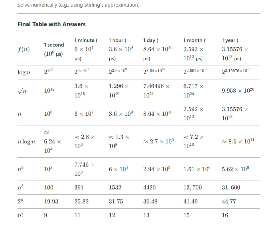
Problem 1-1: Comparison of Running Times

Question:
For each function ( f(n) ) and time ( t ) in the following table, determine the largest size ( n ) of a problem that can be solved in time ( t ), assuming that the algorithm to solve the problem takes ( f(n) ) microseconds.

Part 1: Illustration of Insertion Sort

Let's illustrate the operation of Insertion Sort on the array initially containing the sequence:
⟨31, 41, 59, 26, 41, 58⟩.

Insertion Sort Algorithm

Insertion Sort works by iteratively inserting each element into its correct position in the sorted portion of the array.

---

Step-by-Step Execution

1. Initial Array:
   [31, 41, 59, 26, 41, 58]

2. After 1st Iteration (i = 1):

   • The first element 31 is already in the sorted portion.
   • Sorted portion: [31]
   • Array: [31, 41, 59, 26, 41, 58]

3. After 2nd Iteration (i = 2):

   • Insert 41 into the sorted portion [31].
   • 41 is greater than 31, so it stays in place.
   • Sorted portion: [31, 41]
   • Array: [31, 41, 59, 26, 41, 58]

4. After 3rd Iteration (i = 3):

   • Insert 59 into the sorted portion [31, 41].
   • 59 is greater than 41, so it stays in place.
   • Sorted portion: [31, 41, 59]
   • Array: [31, 41, 59, 26, 41, 58]

5. After 4th Iteration (i = 4):

   • Insert 26 into the sorted portion [31, 41, 59].
   • 26 is smaller than 59, 41, and 31, so it moves to the front.
   • Sorted portion: [26, 31, 41, 59]
   • Array: [26, 31, 41, 59, 41, 58]

6. After 5th Iteration (i = 5):

   • Insert 41 into the sorted portion [26, 31, 41, 59].
   • 41 is equal to the last 41, so it stays in place.
   • Sorted portion: [26, 31, 41, 41, 59]
   • Array: [26, 31, 41, 41, 59, 58]

7. After 6th Iteration (i = 6):

   • Insert 58 into the sorted portion [26, 31, 41, 41, 59].
   • 58 is smaller than 59, so it moves before 59.
   • Sorted portion: [26, 31, 41, 41, 58, 59]
   • Array: [26, 31, 41, 41, 58, 59]

---

Final Sorted Array:

[26, 31, 41, 41, 58, 59]

---

Part 2: Loop Invariant for SUM-ARRAY

The SUM-ARRAY procedure computes the sum of the numbers in the array A[1 : n]. Here is the procedure:

SUM-ARRAY(A, n)
sum = 0
for i = 1 to n
sum = sum + A[i]
return sum

Loop Invariant

A loop invariant is a condition that is true before and after each iteration of the loop. For the SUM-ARRAY procedure, the loop invariant is:

At the start of each iteration of the for loop, the variable sum contains the sum of the elements in the subarray A[1 : i-1].

---

Proof of Correctness Using Loop Invariant

1. Initialization:

   • Before the first iteration (i = 1), the subarray A[1 : 0] is empty.
   • The variable sum is initialized to 0, which is the sum of an empty array.
   • Thus, the loop invariant holds before the first iteration.

2. Maintenance:

   • Assume the loop invariant holds at the start of the i-th iteration, i.e., sum contains the sum of A[1 : i-1].
   • During the i-th iteration, sum is updated to sum + A[i].
   • After the update, sum contains the sum of A[1 : i].
   • Thus, the loop invariant holds at the start of the next iteration.

3. Termination:

   • The loop terminates when i = n + 1.
   • At this point, the loop invariant states that sum contains the sum of A[1 : n].
   • The procedure returns sum, which is the correct sum of all elements in the array.

---

Conclusion

The loop invariant ensures that the SUM-ARRAY procedure correctly computes the sum of the numbers in the array A[1 : n]. By the properties of initialization, maintenance, and termination, the procedure is proven to be correct.

Gyver Tc, [2/17/2025 1:47 PM]

Part 1: Insertion Sort for Monotonically Decreasing Order

To modify the Insertion Sort algorithm to sort in monotonically decreasing order, we need to change the comparison condition. Instead of inserting elements into the correct position in an increasing sequence, we insert them into the correct position in a decreasing sequence.

Pseudocode for Decreasing Insertion Sort

INSERTION-SORT-DECREASING(A)
for j = 2 to A.length
key = A[j]
i = j - 1
// Insert A[j] into the sorted sequence A[1 : j-1] in decreasing order
while i > 0 and A[i] < key
A[i + 1] = A[i]
i = i - 1
A[i + 1] = key

Explanation

• The outer loop iterates over each element in the array.
• The inner loop shifts elements to the right until the correct position for key is found in the decreasing sequence.
• The condition A[i] < key ensures that the sequence remains monotonically decreasing.

---

Part 2: Linear Search Pseudocode and Correctness Proof

Pseudocode for Linear Search

LINEAR-SEARCH(A, x)
for i = 1 to A.length
if A[i] == x
return i
return NIL

Loop Invariant

The loop invariant for the LINEAR-SEARCH algorithm is:

At the start of each iteration of the for loop, the element x does not appear in the subarray A[1 : i-1].

---

Proof of Correctness Using Loop Invariant

1. Initialization:

   • Before the first iteration (i = 1), the subarray A[1 : 0] is empty.
   • By definition, x does not appear in an empty array.
   • Thus, the loop invariant holds before the first iteration.

2. Maintenance:

   • Assume the loop invariant holds at the start of the i-th iteration, i.e., x does not appear in A[1 : i-1].
   • During the i-th iteration, the algorithm checks if A[i] == x.
     • If A[i] == x, the algorithm returns i, and the loop terminates.
     • If A[i] != x, the loop invariant holds for the next iteration (i + 1).
   • Thus, the loop invariant is maintained.

3. Termination:

   • The loop terminates when either x is found or i exceeds A.length.
   • If x is found, the algorithm returns the correct index.
   • If x is not found, the algorithm returns NIL, which is correct because the loop invariant ensures that x does not appear in A[1 : A.length].

---

Part 3: Adding Two n-Bit Binary Integers

The problem involves adding two n-bit binary integers stored in arrays A and B and storing the result in an (n + 1)-bit array C.

Pseudocode for ADD-BINARY-INTEGERS

ADD-BINARY-INTEGERS(A, B, n)
let C[0 : n] be a new array
carry = 0
for i = n - 1 downto 0
sum = A[i] + B[i] + carry
C[i + 1] = sum % 2 // Store the least significant bit
carry = sum // 2 // Update the carry
C[0] = carry
return C

Explanation

1. Initialization:

   • Create a new array C of size n + 1 to store the result.
   • Initialize carry to 0.

2. Loop:

   • Iterate from the least significant bit (LSB) to the most significant bit (MSB).
   • Compute the sum of A[i], B[i], and carry.
   • Store the LSB of the sum in C[i + 1].
   • Update the carry for the next iteration.

3. Final Carry:

   • After the loop, store the final carry in C[0].

4. Return:

   • Return the array C containing the sum.

---

Example

Input:
A = [1, 0, 1, 1] (binary number 1011, decimal 11)
B = [1, 1, 0, 1] (binary number 1101, decimal 13)
n = 4

Execution:

• Iteration 1: sum = 1 + 1 + 0 = 2, C[4] = 0, carry = 1
• Iteration 2: sum = 1 + 0 + 1 = 2, C[3] = 0, carry = 1
• Iteration 3: sum = 0 + 1 + 1 = 2, C[2] = 0, carry = 1
• Iteration 4: sum = 1 + 1 + 1 = 3, C[1] = 1, carry = 1
• Final Carry: C[0] = 1

Output:
C = [1, 1, 0, 0, 0] (binary number 11000, decimal 24)

---

Summary

1. Insertion Sort for Decreasing Order: Modify the comparison condition to sort in decreasing order.
2. Linear Search: Use a loop invariant to prove correctness.
3. Binary Addition: Implement a procedure to add two n-bit binary integers and store the result in an (n + 1)-bit array.

Shortest path algorithms have a wide range of practical applications across various fields. Here are some key examples:

1. Navigation Systems:

   • GPS and Maps: Used in GPS devices and mapping applications (like Google Maps) to find the quickest route between two locations, taking into account traffic conditions and road networks.

2. Network Routing:

   • Internet Routing: Determines the most efficient path for data packets to travel across the internet, ensuring faster and more reliable communication.
   • Telecommunications: Optimizes the routing of phone calls and messages through networks to minimize latency and costs.

3. Transportation and Logistics:

   • Public Transportation: Helps in planning the shortest and most efficient routes for buses, trains, and other public transit systems.
   • Delivery Services: Used by companies like FedEx and UPS to optimize delivery routes, reducing fuel consumption and delivery times.

4. Robotics and Autonomous Vehicles:

   • Robot Navigation: Enables robots to find the shortest path in an environment, avoiding obstacles and optimizing their movements.
   • Self-Driving Cars: Assists in route planning and navigation, ensuring safe and efficient travel.

5. Supply Chain Management:

   • Warehouse Operations: Optimizes the movement of goods within warehouses to ensure quick and efficient retrieval and storage.
   • Inventory Distribution: Determines the most efficient routes for distributing products from warehouses to retail stores.

6. Emergency Response:

   • First Responders: Helps emergency vehicles (ambulances, fire trucks, police) find the quickest route to an emergency site.
   • Evacuation Planning: Assists in creating evacuation plans for buildings or areas during emergencies, ensuring safe and efficient evacuation routes.

7. Social Networks:

   • Friend Recommendations: Analyzes the shortest path between individuals in a social network to suggest potential friends or connections.
   • Influence Spread: Studies how information or influence spreads through a network, identifying key nodes for efficient dissemination.

8. Urban Planning:

   • Infrastructure Development: Assists in planning the layout of roads, bridges, and public transportation systems for optimal connectivity and efficiency.

9. Healthcare:

   • Patient Transport: Optimizes routes for transporting patients within large hospital complexes.
   • Medical Supply Distribution: Ensures efficient delivery of medical supplies to healthcare facilities.

These applications showcase the versatility and importance of shortest path algorithms in solving real-world problems efficiently. If you have any more questions or need further details, feel free to ask! 😊