DL- MNIST 데이터

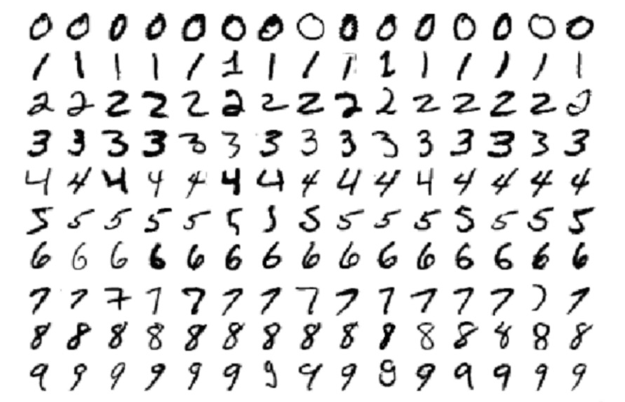
📙 MNIST데이터로 DL과정 복습해보기.

import tensorflow as tf

mnist = tf.keras.datasets.mnist

(x_train, y_train),(x_test,y_test) = mnist.load_data()
x_train, x_test = x_train/ 255.0, x_test / 255.0   
# 픽셀 max가 255. 255로 나눈 것은 minmax scaler쓴 것과 비슷

One-hot Encoding

• loss함수를 sparse_categorical_crossentropy로 설정하면 같은효과. 저절로 onehot encoding 해주는 효과가 난다.
  

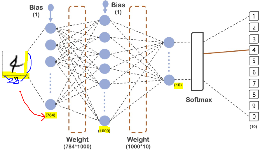
✏28x28을 하나의 열로 펼치면 784. --> 1000개의 노드를 거쳐 0~9, 10개로 나아가는 과정.
-->그 후 sparse_categorical_crossentropy을 거쳐 답이 출력.

model = tf.keras.models.Sequential([
    tf.keras.layers.Flatten(input_shape=(28,28)), #flatten: input shape nXn으로 주면 1열로 펼쳐줌
    tf.keras.layers.Dense(1000,activation='relu'), #은닉층 lelu
    tf.keras.layers.Dense(10,activation='softmax')
])
    
model.compile(optimizer='adam',
              loss='sparse_categorical_crossentropy',
              metrics=['accuracy']) #학습 중 accuracy 반환

model.summary()

Model: "sequential"
_________________________________________________________________
 Layer (type)                Output Shape              Param #   
=================================================================
 flatten (Flatten)           (None, 784)               0         
                                                                 
 dense (Dense)               (None, 1000)              785000    
                                                                 
 dense_1 (Dense)             (None, 10)                10010     
                                                                 
=================================================================
Total params: 795,010
Trainable params: 795,010
Non-trainable params: 0
_________________________________________________________________

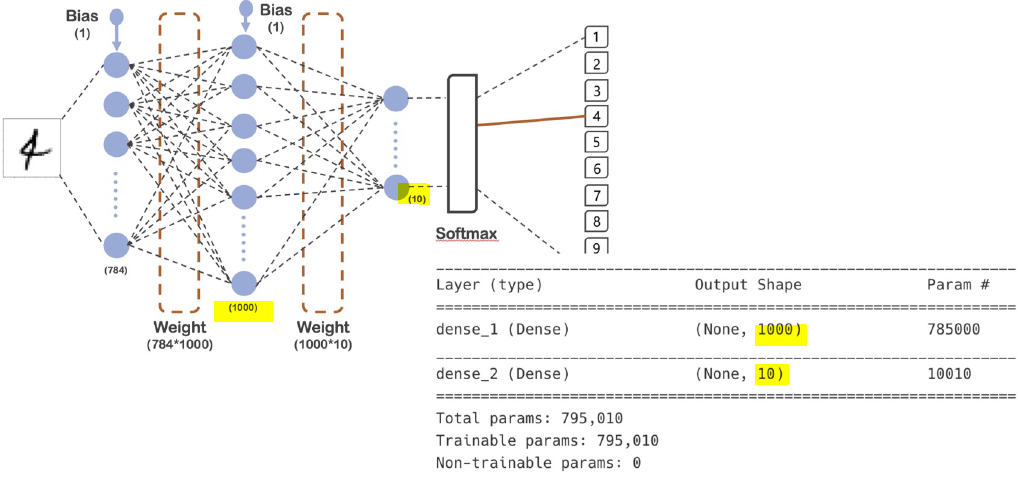
코드와 모델 일치

%%time

hist = model.fit(x_train,y_train,validation_data=(x_test,y_test),epochs=10,batch_size=100,verbose=1) #verbose : 학습하는 동안의 상황을 그래픽하게 표현
#데이터 한 묶음에 100개씩 600 묶음.
#소요 시간 3s : 배치 사이즈 100으로 하고, 600묶음의 데이터 학습시키는 하나의 epoch에 걸리는 시간 3초.

Epoch 1/10
600/600 [==============================] - 2s 3ms/step - loss: 0.0063 - accuracy: 0.9981 - val_loss: 0.0808 - val_accuracy: 0.9793
Epoch 2/10
600/600 [==============================] - 2s 4ms/step - loss: 0.0067 - accuracy: 0.9979 - val_loss: 0.0817 - val_accuracy: 0.9815
Epoch 3/10
600/600 [==============================] - 2s 3ms/step - loss: 0.0071 - accuracy: 0.9978 - val_loss: 0.0781 - val_accuracy: 0.9815
Epoch 4/10
600/600 [==============================] - 2s 4ms/step - loss: 0.0060 - accuracy: 0.9982 - val_loss: 0.0862 - val_accuracy: 0.9817
Epoch 5/10
600/600 [==============================] - 3s 4ms/step - loss: 0.0074 - accuracy: 0.9976 - val_loss: 0.0914 - val_accuracy: 0.9784
Epoch 6/10
600/600 [==============================] - 3s 4ms/step - loss: 0.0034 - accuracy: 0.9991 - val_loss: 0.0767 - val_accuracy: 0.9822
Epoch 7/10
600/600 [==============================] - 2s 4ms/step - loss: 0.0016 - accuracy: 0.9996 - val_loss: 0.0697 - val_accuracy: 0.9842
Epoch 8/10
600/600 [==============================] - 2s 4ms/step - loss: 0.0020 - accuracy: 0.9995 - val_loss: 0.1102 - val_accuracy: 0.9784
Epoch 9/10
600/600 [==============================] - 2s 4ms/step - loss: 0.0132 - accuracy: 0.9956 - val_loss: 0.0831 - val_accuracy: 0.9823
Epoch 10/10
600/600 [==============================] - 2s 4ms/step - loss: 0.0037 - accuracy: 0.9988 - val_loss: 0.0797 - val_accuracy: 0.9840
CPU times: total: 1min 40s
Wall time: 22.5 s

import matplotlib.pyplot as plt
%matplotlib inline
plot_target = ['loss','val_loss','accuracy','val_accuracy']

plt.figure(figsize=(12,8))

for each in plot_target:
    plt.plot(hist.history[each],label=each)
    
plt.legend()
plt.grid()
plt.show()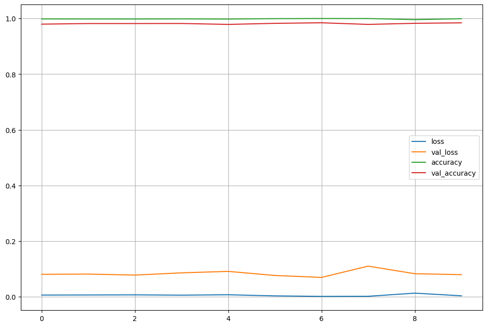

validation loss, (training)loss 간에 간격이 조금 있어보이긴 하나, (training) accuracy 거의 100에 근접.

score = model.evaluate(x_test,y_test)
print('Test loss:',score[0])
print('test accuracy:',score[1])

313/313 [==============================] - 1s 2ms/step - loss: 0.0797 - accuracy: 0.9840
Test loss: 0.07967743277549744
test accuracy: 0.984000027179718

➡accuracy 98%

import numpy as np

predicted_result = model.predict(x_test)
predicted_result[0]   
# 가장 높은 값 max = 1.0000000e+00, '7'

array([4.2500915e-13, 4.3836195e-15, 4.6376505e-12, 4.0975870e-08,
       4.1196887e-18, 3.5640494e-14, 4.5751641e-20, 1.0000000e+00,
       1.9685302e-13, 3.2595003e-11], dtype=float32)

predicted_labels = np.argmax(predicted_result,axis=1) 
predicted_labels[:10]

array([7, 2, 1, 0, 4, 1, 4, 9, 5, 9], dtype=int64)

- 잘못 예측한 경우 확인

예측 확률이 높은 경우 해당 값을 선택한다.

• np.argmax : 각 행(axis=1), 열(axis=0)에서의 최대값의 인덱스를 반환한다.

# 정답 확인
y_test[:10]

array([7, 2, 1, 0, 4, 1, 4, 9, 5, 9], dtype=uint8)

wrong_result =[]

for n in range(0,len(y_test)):
    if predicted_labels[n] !=y_test[n]:
        wrong_result.append(n)
        
len(wrong_result) 

160

틀린 데이터 총 160개 확인.

import random

samples = random.choices(population = wrong_result,k=16)

plt.figure(figsize=(14,12))

for idx, n in enumerate(samples):
    plt.subplot(4,4,idx+1) # 16개 
    plt.imshow(x_test[n].reshape(28,28),cmap='Greys')
    plt.title('Label:' + str(y_test[n]) + ' | predict :'+ str(predicted_labels[n]))
    plt.axis

---

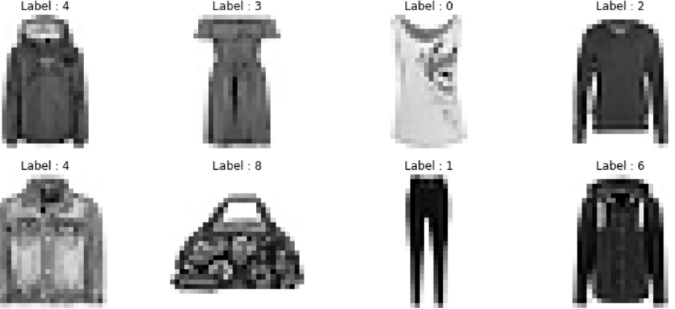
📙MNIST FASHION 데이터

• 숫자로 된 MNIST데이터 처럼 28*28크기의 패션 관련 10개 종류의 데이터
  

label	종류
0	티셔츠
1	바지
2	스웨터
3	드레스
4	코트
5	샌들
6	셔츠
7	운동화
8	가방
9	부츠

# 데이터 읽기
fashion_mnist = tf.keras.datasets.fashion_mnist

(x_train, y_train),(x_test,y_test) = fashion_mnist.load_data()
x_train, x_test = x_train/255, x_test/255

Downloading data from https://storage.googleapis.com/tensorflow/tf-keras-datasets/train-labels-idx1-ubyte.gz
32768/29515 [=================================] - 0s 0us/step
40960/29515 [=========================================] - 0s 0us/step
Downloading data from https://storage.googleapis.com/tensorflow/tf-keras-datasets/train-images-idx3-ubyte.gz
26427392/26421880 [==============================] - 1s 0us/step
26435584/26421880 [==============================] - 1s 0us/step
Downloading data from https://storage.googleapis.com/tensorflow/tf-keras-datasets/t10k-labels-idx1-ubyte.gz
16384/5148 [===============================================================================================] - 0s 0s/step
Downloading data from https://storage.googleapis.com/tensorflow/tf-keras-datasets/t10k-images-idx3-ubyte.gz
4423680/4422102 [==============================] - 0s 0us/step
4431872/4422102 [==============================] - 0s 0us/step

samples = random.choices(population=range(0,len(y_train)),k=16)

plt.figure(figsize=(14,12))

for idx, n in enumerate(samples):
    plt.subplot(4,4,idx+1)
    plt.imshow(x_train[n].reshape(28,28),cmap='Greys')
    plt.title('Label:' + str(y_train[n]))
    plt.axis('off')
    
plt.show()

모델은 숫자때와 동일한 구조로 두자

model = tf.keras.models.Sequential([
    tf.keras.layers.Flatten(input_shape=(28,28)), 
    tf.keras.layers.Dense(1000,activation='relu'), 
    tf.keras.layers.Dense(10,activation='softmax')
])
    
model.compile(optimizer='adam',
              loss='sparse_categorical_crossentropy',
              metrics=['accuracy']) 

%%time

hist = model.fit(x_train,y_train,validation_data=(x_test,y_test),epochs=10,batch_size=100,verbose=1)

Epoch 1/10
600/600 [==============================] - 2s 4ms/step - loss: 0.4840 - accuracy: 0.8289 - val_loss: 0.4564 - val_accuracy: 0.8366
Epoch 2/10
600/600 [==============================] - 2s 3ms/step - loss: 0.3586 - accuracy: 0.8712 - val_loss: 0.3795 - val_accuracy: 0.8632
Epoch 3/10
600/600 [==============================] - 2s 4ms/step - loss: 0.3227 - accuracy: 0.8815 - val_loss: 0.3816 - val_accuracy: 0.8551
Epoch 4/10
600/600 [==============================] - 2s 4ms/step - loss: 0.2959 - accuracy: 0.8909 - val_loss: 0.3531 - val_accuracy: 0.8700
Epoch 5/10
600/600 [==============================] - 2s 4ms/step - loss: 0.2779 - accuracy: 0.8975 - val_loss: 0.3434 - val_accuracy: 0.8761
Epoch 6/10
600/600 [==============================] - 2s 4ms/step - loss: 0.2617 - accuracy: 0.9031 - val_loss: 0.3193 - val_accuracy: 0.8850
Epoch 7/10
600/600 [==============================] - 2s 4ms/step - loss: 0.2490 - accuracy: 0.9074 - val_loss: 0.3164 - val_accuracy: 0.8887
Epoch 8/10
600/600 [==============================] - 2s 4ms/step - loss: 0.2398 - accuracy: 0.9105 - val_loss: 0.3400 - val_accuracy: 0.8803
Epoch 9/10
600/600 [==============================] - 2s 4ms/step - loss: 0.2260 - accuracy: 0.9166 - val_loss: 0.3273 - val_accuracy: 0.8833
Epoch 10/10
600/600 [==============================] - 2s 4ms/step - loss: 0.2199 - accuracy: 0.9172 - val_loss: 0.3211 - val_accuracy: 0.8886
CPU times: total: 1min 46s
Wall time: 22.5 s

plot_target = ['loss','val_loss','accuracy','val_accuracy']

plt.figure(figsize=(12,8))

for each in plot_target:
    plt.plot(hist.history[each],label=each)
    
plt.legend()
plt.grid()
plt.show()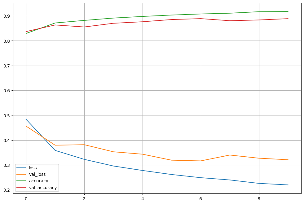

➡training acc는 좋아지지만 val_acc는 다소 정체하는 걸 확인.

score = model.evaluate(x_test,y_test)
print('Test loss :', score[0])
print('Test acc :', score[1])

313/313 [==============================] - 1s 2ms/step - loss: 0.3211 - accuracy: 0.8886
Test loss : 0.3210602104663849
Test acc : 0.8885999917984009

predicted_result = model.predict(x_test)
predicted_labels = np.argmax(predicted_result,axis=1) 
predicted_labels[:10]

array([9, 2, 1, 1, 6, 1, 4, 6, 5, 7], dtype=int64)

y_test[:10]

array([9, 2, 1, 1, 6, 1, 4, 6, 5, 7], dtype=uint8)

# 틀린 데이터 확인
wrong_result =[]

for n in range(0,len(y_test)):
    if predicted_labels[n] !=y_test[n]:
        wrong_result.append(n)
        
len(wrong_result) 

1114

samples = random.choices(population = wrong_result,k=16)
plt.figure(figsize=(14,12))

for idx, n in enumerate(samples):
    plt.subplot(4,4,idx+1)
    plt.imshow(x_test[n].reshape(28,28),cmap='Greys', interpolation='nearest')
    plt.title('Label:' + str(y_test[n]) + ' | predict :'+ str(predicted_labels[n]))
    plt.axis('off')
    
plt.show()

label	종류
0	티셔츠
1	바지
2	스웨터
3	드레스
4	코트
5	샌들
6	셔츠
7	운동화
8	가방
9	부츠