Paper: https://arxiv.org/pdf/2106.06965.pdf
Code: no official github
(필자가 작성한 코드는 최하단에 첨부)
0. Abstract
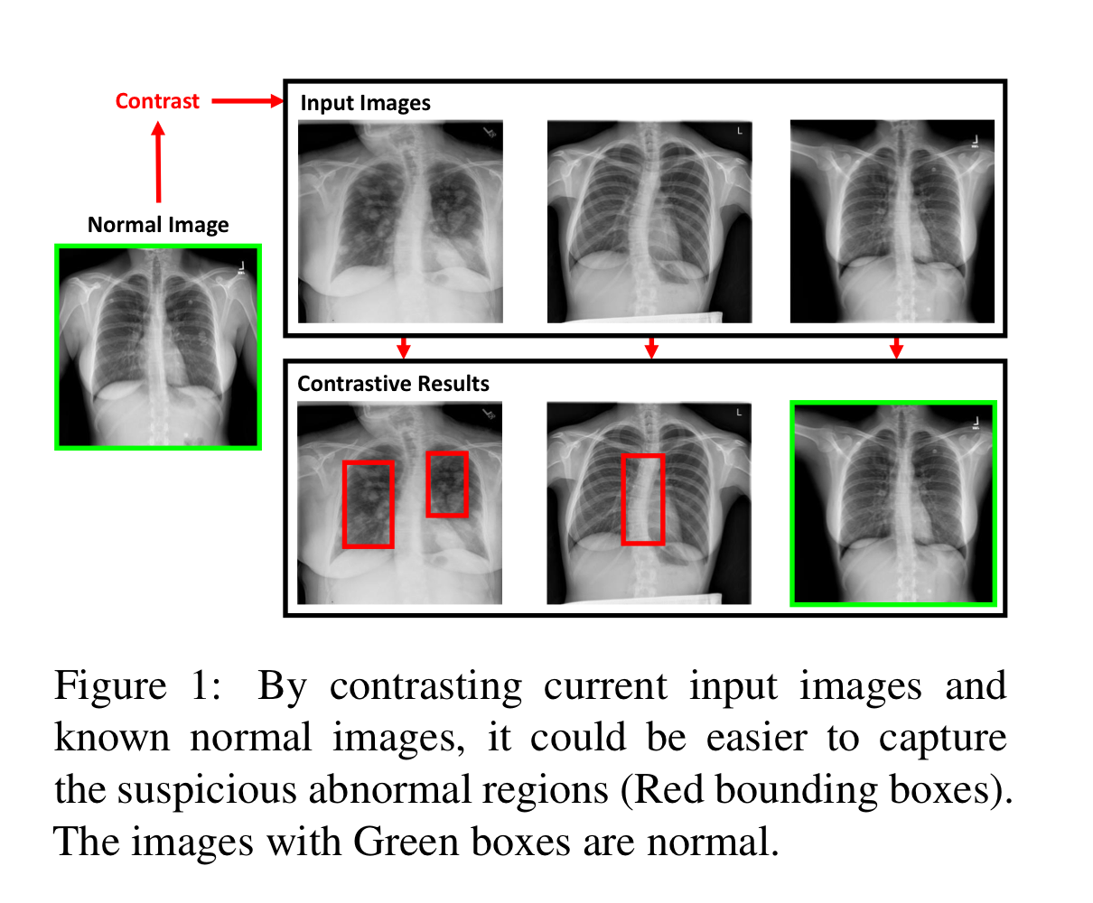
X-ray Report Generation에서 중요한 것은 Abnormal region을 잘 포착하고, 이에 대한 기술을 만들어내는 것입니다.
하지만, X-ray data는 대부분 normal region으로 이루어져 있기 때문에, 이에 영향을 크게 받아 abnormal region을 제대로 포착하지 못하곤 합니다.
이와 같은 데이터 편향을 다루기 위해 저자들은 input image와 normal image간의 contrastive information을 비교하는 모델인 Contrastive Attention(CA) Model을 제안합니다.
이를 통해 abnormal region을 더 잘 포착할 수 잇었으며, 더 정확한 description을 반환할 수 있었습니다.
SoTA라곤 합니다만, 제대로 된 벤치마크 체계가 잡혀있지는 않아서..
1. Introduction
X-ray image를 해석하고 이에 대한 report를 기술하는 것은 관련 분야의 전문 지식과 경험이 필요합니다.
딥러닝이 발달함에 따라 chest X-ray report generation system을 구축하는 것은 이런 전문의들의 부담을 한결 덜어줄 수 있습니다.
하지만, 다른 분야와 다르게 Medical 분야에서의 Report는 기존의 데이터들과 특징이 크게 다를 뿐만 아니라, 이미지 또한 아래와 같은 편향이 존재합니다.
- abnormal image보다 normal image가 훨씬 많다.
- input image가 주어졌을 때, normal region이 abnormal region보다 훨씬 넓다.
이런 데이터 편향 때문에 학습 기반 모델들이 폐 병변과 같은 흔치 않은 영역을 포착하기 힘들어 합니다.
그 결과 이미지에 크게 문제가 없다는 정상적인 report를 반환할 확률이 커집니다.
abnormal region을 포착하는 가장 단순한 방법은 X-ray image를 정상 이미지와 비교해 차이점을 따져보는 것입니다.
이런 아이디어를 받아 저자들은 기존의 모델에 통합해 사용할 수 있는 CA Model을 제안합니다.
제안하는 방법의 과정은 아래와 같습니다.
- training dataset으로 부터 normal images 집합을 구축합니다.
- 투입된 input image와 가까운 normal image의 우선순위를 구하기 위해 Aggregate Attention을 사용합니다.
- input image와 우선순위를 이용해 정제한 normal images 간의 common features를 추출하기 위해 Differentiate Attention을 사용합니다.
- 마지막으로, 이렇게 얻은 common features를 input image의 visual features에서 빼줍니다.
즉, 이렇게 얻은 visual features는 normal image와의 차이점을 강조한 Contrastive information으로 활용할 수 있게 됩니다.
평가는 IU Dataset, MIMIC-CXR Dataset에 대해 평가했으며, Human Evaluation과 automatic metrics 두 부분에서 좋은 결과를 보였습니다.
특히, CA를 사용한 모델의 경우 베이스라인 모델보다 14%~17%가량 성능이 좋아졌습니다.
2. Related Work
2.1. Image Captioning
Image Captioning을 위한 Encoder-Decoder 모델이 많이 개발됐지만, 애초에 이미지의 두드러진 특징만을 묘사할 뿐만 아니라, 생성된 문장 또한 짧은 경향이 있어 이미지의 풍부한 정보를 모두 표현하기란 어려웠습니다.
최근에는 visual paragraph(계층구조)를 활용해 더욱 긴 문장을 생성하는 방법이 각광을 받았었습니다.
하지만, 역시 Medical 분야에서는 이런 계층모델도 normal description만 반환하는 등 제대로 이미지를 포착하지 못하는 모습을 보였습니다.
2.2. Chest X-ray Report Generation
여러 모델들이 등장했지만, Yuan et al, (2019)는 medical concepts Decoder에 사용해 더 나은 report를 생성할 수 있게끔 유도했습니다.
뿐만 아니라 Xue et al.(2018)은 multimodal recurrent model을 이용해 문장 간 맥락이 일치하게끔 학습시켰습니다.
Multimodal recurrent model with attention for automated radiology report generation
Miura et al. (2021)은 사실 정보의 완성과 생성 레포트의 일치를 위한 방법인 Exact Entity Match Reward / Entailing Entity Match REward를 제안해, Clinical accuracy를 상당히 크게 개선했습니다.
Improving Factual Completeness and Consistency of Image-to-Text Radiology Report Generation
이외에도 강화학습을 사용하거나, 의학 지식 그래프를 활용할 수 있습니다만, 당연히 부정확한 결과들을 다수 도출했습니다.
2.3. Contrastive Learning
저자들이 제안하는 CA model과 제일 관련있는 분야는 contrastie learning 분야입니다.
생성 모델 분야에 굉장히 널리 쓰이는..
해당 방법은 주로 모델이 각각의 이미지에 대해 유사한 이미지끼리는 유사한 image representation을, 다른 이미지끼리는 다른 image representation을 생성하게끔 강제하는 방법입니다.
즉, 이미지의 embedding space에서 클래스들이 잘 나뉘게끔.
Image Captioning 분야에서는 Dai and Lin이 이 학습 방법을 도입해 추가적인 이미지로부터 contrastive information을 추출, caption 생성의 distinctiveness를 증진했습니다.
이외에도 사람의 재인식과 요약에 쓰이는 contrastive attention mechanism이나, 사람과 배경간의 차이를 포착하기 위해 segmentation mask를 활용하는 등의 연구가 있었습니다.
3. Apporach
3.1. Problem Formulation
- Input : Image
- Output : coherent report
캡셔닝에는 주로 Image Encoder와 Report Decoder를 사용합니다.
세세한 내용은 미뤄두고, 본 논문에서 저자들은 Image Encoder로 Resnet-50을 사용해 visual features를 뽑아냅니다.
Convolution layer의 최종 output(즉, visual feature)은 아래와 같이 나타낼 수 있습니다.
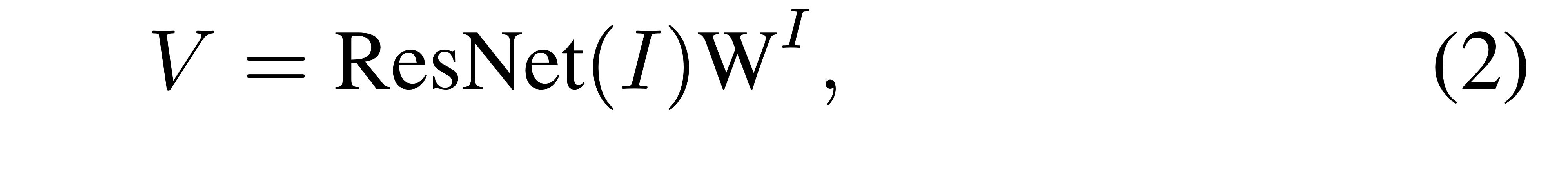
이 때, ResNet(I)는 차원입니다.
이렇게 나온 Feature를 Linear 모델 (즉, 를 활용해 차원으로 감소시킵니다.
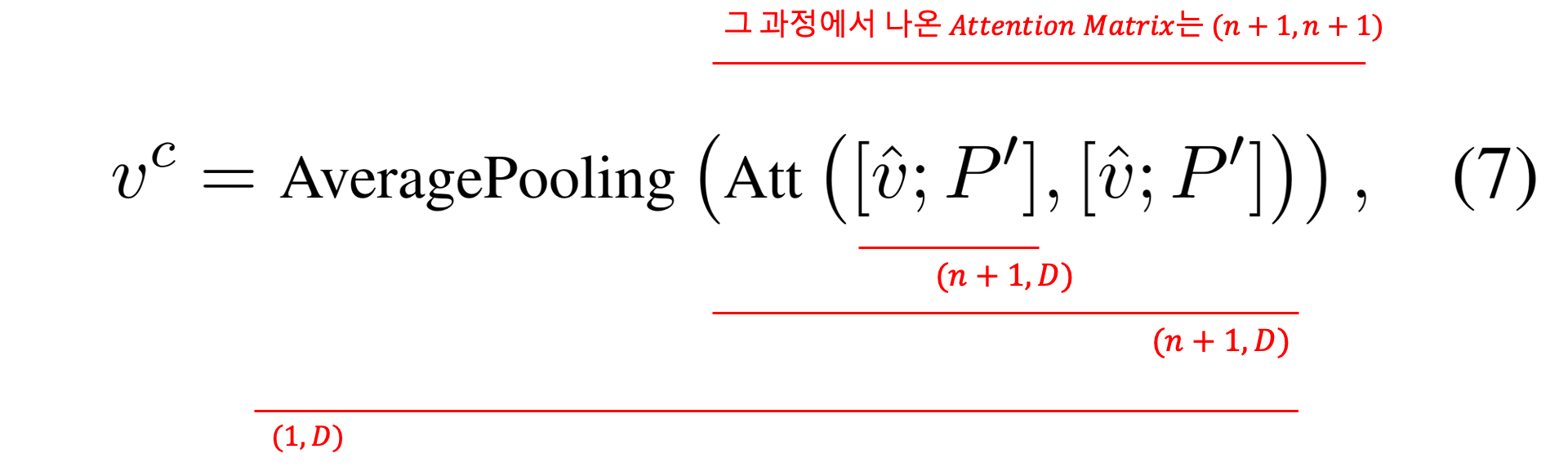
그 후, AveragePooling을 활용해 global visual feature를 얻습니다.
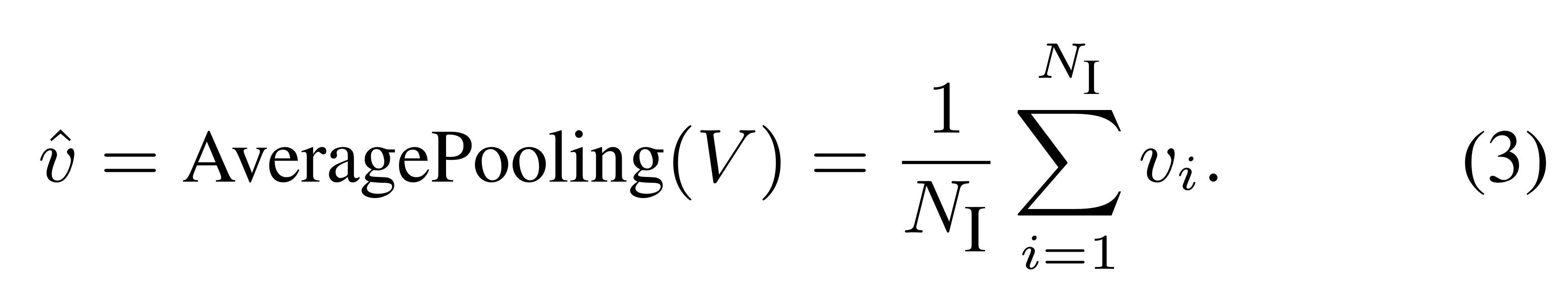
즉, (7x7=)49개의 point를 따라 평균내서 차원의 global features를 얻습니다.
결과적으로 의 visual features와 의 global visual feature
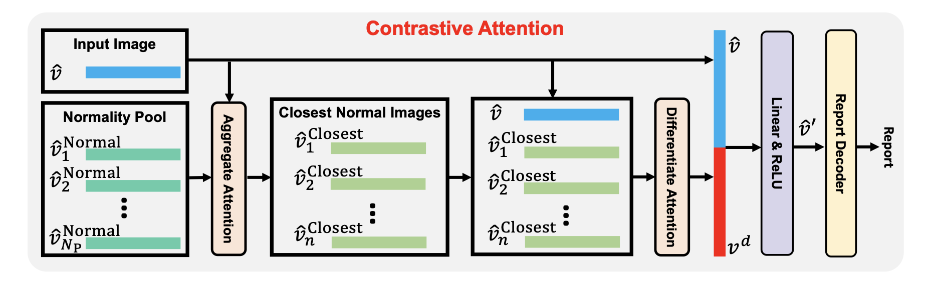
3.2. Constrastive Attention
CA를 구현하기 위해 우선 normal image의 feature를 모아놓은 pool이 필요합니다.
즉,

본 논문에서는 1000개를 랜덤하게 추출.
특히, 각각의 벡터는 위에서 말한 global visual feature로, 차원입니다.
그 후, 아래 그림과 같이 Aggregate Attention과 Differentiate Attention을 적용해 Normality pool 와 input image의 global visual feature인 contrastive information을 뽑습니다.
3.2.1. Aggregate Attention
Normality Pool 에는 모두 정상 이미지만 있기 때문에 이들 간에 중요도를 파악할 수는 없습니다.
하지만, Input Image와 확연하게 다른 Normal Image가 존재하기 때문에 이런 이미지들에 대해서는 가중치를 낮게 줄 필요가 있습니다.
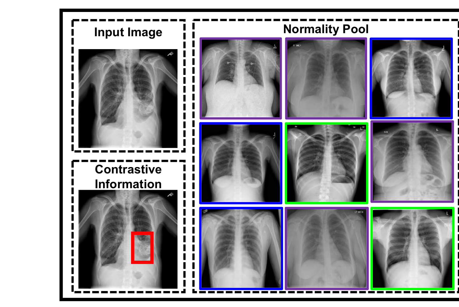
위 그림에서 보라색 박스 = Noisy Normal Image
가령 각도나, 방향이나, 주어진 영역이나..
이와 같은 Normal Image를 사용할 경우 모델이 정확한 abnormal region을 포착하는 것이 힘들어질 수 있습니다.
위와 같은 관찰로부터 영감을 받아, 저자들은 Aggregated Attention을 이용해 input image와 가까운 normal image에는 가중치를 주고, 반대의 경우 가중치를 덜 주는 방법을 고안했습니다.
이에는 어텐션을 활용하는데, 기본적으로 dot-product attention을 사용할 경우 아래와 같이 식을 전개할 수 있습니다.
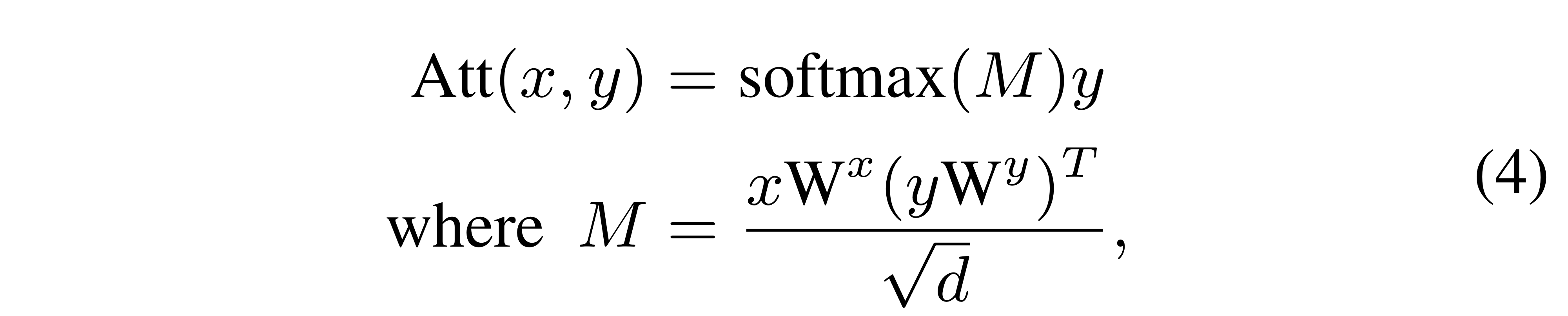
.
즉,
x가 Query, y가 Key, Value 역할.
편의 상 Embedding 차원과 의 차원을 로 통일한듯(굳이 같을 필요는 없긴 함).
단, 같기 때문에 에서 에 대한 Value matrix가 필요 없는 것.
위와 같이 정의하면, 이전에 언급한 global input features 와 Normal Image Pool 간에 어텐션을 계산할 수 있게 됩니다.

즉, 결과물로는 차원의 벡터가 나옵니다.
간단히 말하면, 위의 벡터 는 개의 normality images 들에 대한 가중합을 담고 있는 벡터입니다.
(Attention Weight 을 weight로, 그리고 Pool 내에 있는 normal image들을 value로).
애초에 위와같은 어텐션 과정 자체가 벡터 와 normality Pool 의 원소들인 과 유사도를 구하는 것이기 때문에, input image와 normal image 간의 유사도를 구해 랭킹을 부여할 수 있게 됩니다(뭐 실제로 사용하는 결과 값은 이에 대한 가중합이지만..).
위의 과정은 단순한 내적과 softmax지만, 이미 내적에 벡터 간(즉, global input feature와 global normal feature 간) 유사도 개념이 포함되어 있을 뿐만 아니라, 위에서 학습 가능한 를 통해 input image와 유사한 normal image는 더 높은 attention weight를 갖게 됩니다.
단, 저자들은 각기 다른 Parameter()들을 갖는 여러 개의 Aggregate-Attention을 개 사용했다고 합니다(성능 향상을 위해서).
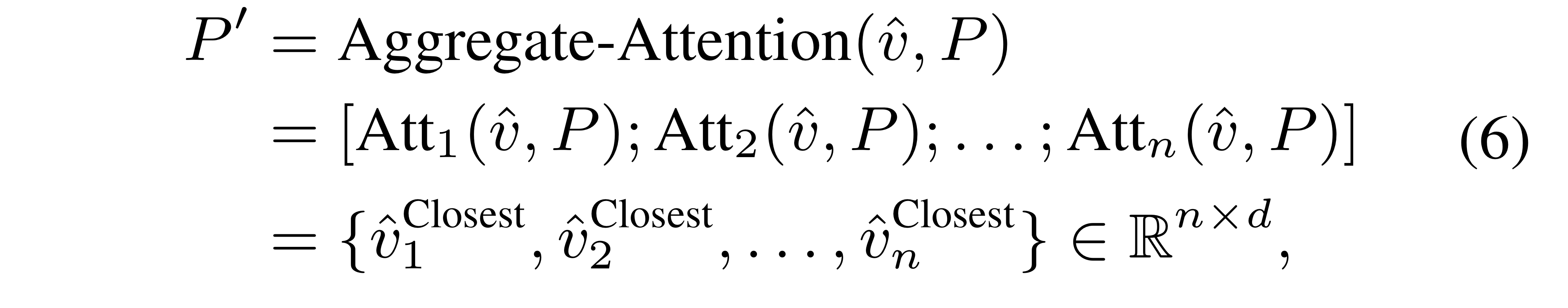
결과적으로 차원의 가 나옵니다.
concat입니다.
by research "structured self-attentive sentence embedding"
위의 의 결과를 통해 전체 input images들에 대해 가까운 normal images를 알 수 있게 됩니다.
아마 의 단순 결과인 vector 로는 그저 (input weighted sum Normal images)만 얻을 수 있는 거지만, 이 과정에서 얻어진 Weight matrix 을 통해서 input image와 normal image 간의 유사도를 알 수 있다고 생각하는 게 타당할 것 같습니다.
단, 위에서도 말햇듯 실제로 사용하는 건 모든 normal images의 유사도와 정보가 혼합된 closest normal images 를 사용합니다 !
다만, 뭐 연산량 등의 문제로 형태의 local feature sequence를 attention에 사용하는 기존의 Image-Attention 기법들과 다르게, 저자들은 형태의 global feature를 사용하게 됩니다.
이를 사용한 Attention을 진행하기 때문에 input image와 normal image간의 유사도도 global 관점에서만 구해지고(전체적인 골격 구조나 이미지 맥락 정도..?),local(specific)한 관점에서 유사한 normal image는 구하기 힘듭니다.
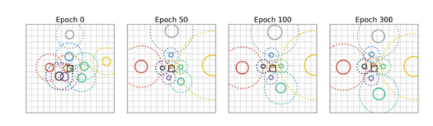
다행이도, 저자들은 위와 같이 Attention을 여러 개 구축함으로써 (마치 Multi-head Attention 처럼) 각 Attention 모듈이 이미지의 각기 다른 parts 중심의 유사도를 파악할 수 있었다고 합니다.
이게 어떻게 되는 지는 정확히 기술한 바 없지만, 학습 과정에서 유리한 방향으로 작동하기 위해 모델이 Attention head가 주목하는 범위를 다양하게 잡은 것으로 이해하면 될 것 같습니다(아래처럼). : [논문리뷰] On The Relationship Between Self-Attention and Convolution Layers
3.2.2. Diffrentiate Attention
위의 Aggregate Attention 과정에서는 현재의 input image와 normal images들이 얼마나 유사한지 구할 수 있었습니다.
이렇게 구한 closest normal images와 input image 사이의 contrastive information을 학습하기 위해 저자들이 행한 프로시저는 아래와 같습니다.
- 두 이미지 사이에 유사성(common information)을 포착한다.
- 위의 common information을 input image에서 뺀다.
당연히 위의 image는 의 global image feature로 생각.
그러면, 어떻게 차원의 input image와 차원의 normal images(normality Pool) 간의 공통 정보 를 추출할까요?
이를 위해 저자들은 Aggregate Attention 과정에서 행했던 것과 같은 dot-product attention을 사용합니다.
단, global input features 와 normality Pool 간의 Attention을 했던 것과는 다르게, Differentiate Attention에서는 와 이전 파트에서 구했던 closest normal images 를concat으로 연결한 다음, self-attention을 진행하게 됩니다.

차원을 나타내면 아래와 같습니다.
위와 같은 Attention 연산의 결과로, global input features 와 closest normal images 간 유사도를 이용, common information을 포착할 수 있게 됩니다.
위의 의 각 는 input images와 유사도가 반영된 normality Pool입니다(가중합 된 거라 ).
에 따라서 모델이 집중하는 이미지 위치가 다릅니다.
즉, (매우 간단하게 예를 들어) 는 input image와 골격이 유사한 normal images 정보, 는 input image와 병변이 유사한 normal images...
즉, 이미 input image와 유사한 다차원적인 개의 closest normal images들과 input image**를 묶어서 self-attention하는 것이기 때문에, 어느 정도 input image와 normal images 간의 유사한 정보를 고려하는 연산이라고 볼 수 있습니다.
다만 아무리 closes normal images들만 뽑아왔다고 한들, input image와의 common information을 뽑는데 를 다이렉트로 연산하지 않고 위와 같이 Self-Attention을 진행해서 Average Pooling을 하는 이유는 잘 모르겠습니다.
즉, Input Image <-> Closest Normal Images 외에도 Closes Normal Images 1 <-> Closest Normal Images 2 간의 유사도까지 계산해 반영한 것인데, 직관적으로 옳다기 보단 더 많은 정보를 담고, 더 나은 성능을 보였기 때문이 아닐까 추측해봅니다.
아무튼, 기존의 global input feature 에서 common information 를 빼서 아래와 같이 최종적인 (contrastive input information) 를 얻을 수 있게 됩니다.

마지막으로 기존 input global feature 와 최종적인 constrastive input feature 를 concat해, Linear projection 해줌으로써 모든 정보가 가미된 global feature 를 얻습니다(식(9)).
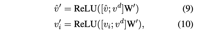
마찬가지로 기존 input local features 도 각각 constrastive input feature 와 concat해 Linear projection 해줘서 새로운 image features 를 얻습니다(식(10)).
아무리 contrastive input image라 할 지라도 original input image도 같이 넣어주는 게 정보 손실이 적겠죠(contrastive 과정이 완벽할 수는 없으니까, 혹은 그냥 경험적인 직감).
두 feature를 concat하게 되면 기존의 image feature dim인 에서 로 증가하기 때문에, 위 식에서 나타난 는 로 설정해 다시 차원으로 맞춰줍니다.
그렇게 얻은 와 는 기존의 image feature인 , 를 대체하게 됩니다.
이렇게 얻은 contrastive features를 사용하면 다른 모델보다 abnormal region을 더 강조해 report generation을 행하는 모습을 보였다고 합니다 !
4. Experiments
4.1. Dataset & Baseline & Settings
https://arxiv.org/pdf/2106.06965.pdf
Dataset & Baseline
- Dataset : MIMIC-CXR, IU X-ray
- MIMIC : 368,960 in the training set, 2,991 in the validation set and 5,159 in the test set
- Baseline : pass
Settings
-
= 512
-
= 6 (Aggregate Attention 개수)
-
= 1000 (사용할 Normal Image Pool)
-
Chexpert-pretrained Resnet-50
- Final feature : 2048
- Final project : 2048 -> 512
- 베이스라인 모델들에 대해 일절 건드리지 않았다고 함.
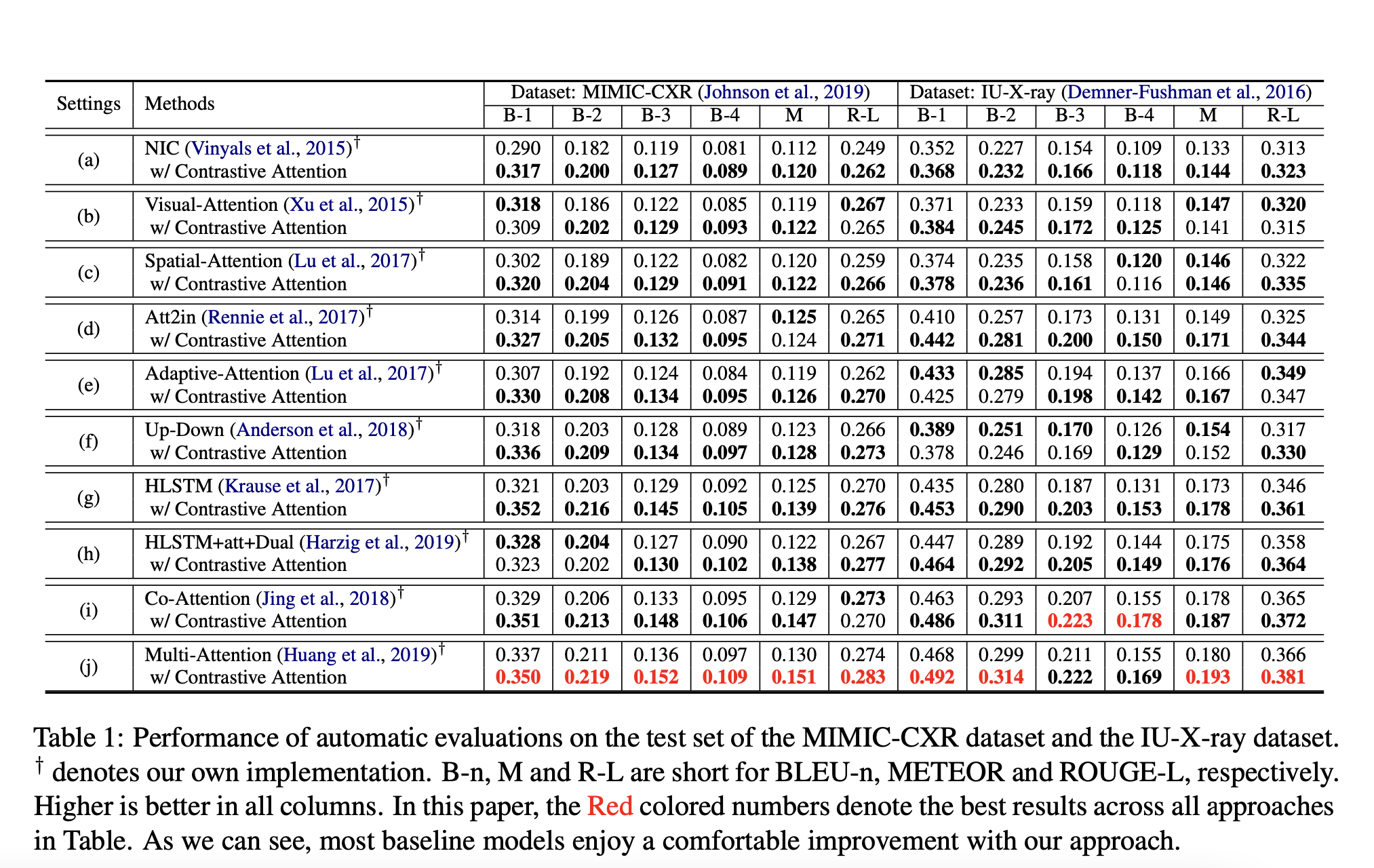
기본적인 성능은 좀 낮지만, 대부분의 베이스라인에 대해 성능 향상을 불러일으켰다는 점이 고무적인 것 같다.
A. Code(Pytorch)
저자와 다를 수 있으며, 정리는 생략했습니다.
from pydantic import annotated_types
import torch
import torch.nn as nn
import numpy as np


# 기존의 모델에 Contrastive Attention을 적용해봅시다.

class ContraAtt(nn.Module):
    def __init__(self, cfg):
        """
        att_type : dot product(Default) or Bi-Linear
        embed_dim : same to input dim(Default)
        """

        super(ContraAtt, self).__init__()
        self.cfg = cfg
        self.att_type = cfg.MODEL.CONTRA_ATT_TYPE
        self.att_dim = cfg.MODEL.ATT_FEATS_DIM # xtransformer : 1024, other : 512
        self.num_heads = cfg.MODEL.CONTRA_ATT_NUM_HEADS # 6 (Default)
        self.aggre_att = AggregatedAttention(self.att_dim, self.num_heads, self.att_type)
        self.diff_att = DifferentiateAttention(self.att_dim, self.att_type)
        self.update_feats = nn.Sequential(
            nn.Linear(in_features=2*self.att_dim, out_features=self.att_dim),
            nn.ReLU()
        )


    def forward(self, input_feats, global_normal_feats):
        """
        input_feats : [196, B, 1024]
        normal_feats : [B, N, 1024]
        """

        src_len = input_feats.shape[0] # 196
        global_input_feats = input_feats.mean(axis=0) # [B, 512]

        closest_normal_feats = self.aggre_att(global_input_feats, global_normal_feats) # [B, 6, 1024]

        common_information = self.diff_att(global_input_feats, closest_normal_feats) # [B, 1, 7, 1024] -- 1 : num of DA heads, 6 : # num of AA heads

        # basic
        # AP
        common_information = common_information.squeeze(1).mean(axis=1) # [B, 1024]

        diff_input_feats = global_input_feats - common_information # [B, 1024]

        # input feats[196, B, 1024] + diff_input_feats[B, 1024]
        # --> [196, B, 1024] + [196, B, 1024] by expand diff_input_feats
        # --> [196, B, 2048]  by concat
        # --> [196, B, 1024]  by update_feats(Linear(2048, 2012))
        diff_input_feats_par = diff_input_feats.unsqueeze(0).expand(src_len, -1, -1) # [196, B, 1024]

        contra_feats = self.update_feats(torch.cat([input_feats, diff_input_feats_par], dim=2)) # [196, B, 1024]

        return contra_feats


class AggregatedAttention(nn.Module): # Aggregated Attention

    def __init__(self, att_dim, num_heads, att_type):
        super(AggregatedAttention, self).__init__()

        self.att_dim = att_dim
        self.num_heads = num_heads
        self.att_type = att_type

        if self.att_type =='dot':
            self.att_blocks = nn.ModuleList([DotAttentionBlock(att_dim) for _ in range(num_heads)])

        if self.att_type =='BiP':
            self.att_blocks = nn.ModuleList([BilinearPoolingAttentionBlock(att_dim) for _ in range(num_heads)])


    def forward(self, global_input_feats, global_normal_feats):
        """
        global_input_feats : [B, 1024]
        global_normal_feats : [B, N, 1024]
        """

        closest_normal_feats = []
        for idx in range(self.num_heads):
            if self.att_type =='dot':
                # [B, query_len, hid_dim] * [B, key_len, hid_dim]
                closest_normal_feat = self.att_blocks[idx](global_input_feats.unsqueeze(1), global_normal_feats) # [B, 1, 1024]

        	closest_normal_feats.append(closest_normal_feat.unsqueeze(0))

        closest_normal_feats = torch.cat(closest_normal_feats) # [n, B, 1, 1024] (n=6)

        closest_normal_feats = closest_normal_feats.permute(1,0,2,3) # [B, n, 1, 1024]
        closest_normal_feats = closest_normal_feats.squeeze(2) # [B, n, 1024]

        return closest_normal_feats

class DifferentiateAttention(nn.Module): # Aggregated Attention

    def __init__(self, att_dim, att_type, num_heads = 1):
        super(DifferentiateAttention, self).__init__()

        self.att_dim = att_dim
        self.att_type = att_type
        self.num_heads = num_heads # Default : 1

        if self.att_type =='dot':
            self.att_blocks = nn.ModuleList([DotAttentionBlock(att_dim) for _ in range(num_heads)])
        if self.att_type =='BiP':
            self.att_blocks = nn.ModuleList([BilinearPoolingAttentionBlock(att_dim) for _ in range(num_heads)])

    def forward(self, global_input_feats, closest_normal_feats):
        """
        input : global_input_feats ([B, hid_dim]), cloasest_normal_feats ([B, n, hid_dim]
        output : diff_att_feats ([B, 1+n, hid_dim]) """


        common_feats = torch.cat([global_input_feats.unsqueeze(1), closest_normal_feats], axis=1) # [B, n+1, hid_dim]

        common_att_feats=[]


        for idx in range(self.num_heads): # default : 1
            if self.att_type =='dot':
                common_att_feat = self.att_blocks[idx](common_feats, common_feats) # [B, n+1, hid_dim]

            common_att_feats.append(common_att_feat.unsqueeze(0))

        common_att_feats = torch.cat(common_att_feats) # [1, B, n+1, hid_dim] (n=6)

        common_att_feats = common_att_feats.permute(1,0,2,3) # [B, 1, n+1, hid_dim]  (1 : DA의 head 개수, n : AA의 head 개수)

        return common_att_feats

class DotAttentionBlock(nn.Module):

    def __init__(self, hid_dim):
        super(DotAttentionBlock, self).__init__()
        self.hid_dim = hid_dim
        self.scale = torch.sqrt(torch.FloatTensor([self.hid_dim])).cuda()
        self.proj_input = nn.Linear(in_features=hid_dim, out_features = hid_dim)
        self.proj_normal = nn.Linear(in_features=hid_dim, out_features=hid_dim)

    def forward(self, global_input_feats, global_normal_feats):
        """
        input : global_input_feats([B, 1 hid_dim]), global_normal_feats([B, N, hid_dim])
        output : closeset_normal_feat([B, 1, hid_dim])
        """

        # for key,value in self.proj_input.named_parameters():

        Q = self.proj_input(global_input_feats) # [B, 1, hid_dim]
        K = self.proj_normal(global_normal_feats) # [B, N, hid_dim]

        # Attention Value
        M = torch.matmul(Q, K.permute(0,2,1))/self.scale # [B, 1, N]

        # Attention map
        attention = torch.softmax(M, dim=-1) # [B, 1, N}
        # Final feature
        closest_normal_feats = torch.matmul(attention, global_normal_feats) # [B, 1, hid_dim] (=[B, 1, N] * [B, N, hid_dim])


        return closest_normal_feats


class BilinearPoolingAttentionBlock(nn.Module):

    def __init__(self, hid_dim):

        super(BilinearPoolingAttentionBlock, self).__init__()

        self.hid_dim = hid_dim
        squeeze_dim = int(hid_dim/2)
        self.squeeze_dim = squeeze_dim

        # self.scale = torch.sqrt(torch.FloatTensor([self.hid_dim])) #.cuda()

        self.proj_input_key = nn.Linear(in_features=hid_dim, out_features = hid_dim)
        self.proj_normal_key = nn.Linear(in_features=hid_dim, out_features= hid_dim)
        self.proj_input_value = nn.Linear(in_features=hid_dim, out_features = hid_dim)
        self.proj_normal_value = nn.Linear(in_features=hid_dim, out_features= hid_dim)

        self.embed1 = nn.Linear(in_features =  hid_dim, out_features = squeeze_dim) # : self.squeeze
        self.embed2 = nn.Linear(in_features = squeeze_dim, out_features = 1)
        self.excitation = nn.Linear(in_features = squeeze_dim, out_features = hid_dim)

        self.relu = nn.ReLU()
        self.sigmoid = nn.Sigmoid()

    def forward(self, global_input_feats, global_normal_feats):
        """
        input : global_input_feats([B, 1 hid_dim]), global_normal_feats([B, N, hid_dim])
        output : closeset_normal_feat([B, 1, hid_dim])
        """
        B, N, hid_dim = global_normal_feats.shape

        # Query - Key Bilinear Pooling
        Q_k = self.proj_input_key(global_input_feats) # [B, 1, hid_dim]
        K = self.proj_normal_key(global_normal_feats) # [B, N, hid_dim]

        ## B_k = [B, N, hid_dim] * [B, N, hid_dim]
        B_k = self.sigmoid(Q_k.expand(-1, N, -1)) * self.sigmoid(K) # expand는 생략해도 무방하나, 직관성을 위해 표기

        # print('Q_k', Q_k.shape) # [B, 1, hid_dim]
        # print('K', K.shape) # [B, N, hid_dim]
        # print('B_k', B_k.shape) # [B, N, hid_dim]

        # embed 1 (squeeze)
        B_k_prime = self.relu(self.embed1(B_k)) # [B, N, hid_dim/2]
        # print('B_k_prime', B_k_prime.shape)

        # spatial attention (beta_s)
        b_s = self.embed2(B_k_prime) # [B, N, 1]
        # print('b_s', b_s.shape)

        beta_s = b_s.softmax(dim=1) # [B, N, 1]
        # print('beta_s', beta_s.shape)

        # channel-wise attention (excitation) (beta_c)

        B_bar = B_k_prime.mean(dim=1) # [B, hid_dim/2]
        # print('B_bar', B_bar.shape)

        b_c = self.excitation(B_bar) # [B, hid_dim]
        beta_c = self.sigmoid(b_c) # [B, hid_dim]
        # print('beta_c', beta_c.shape)


        # Query - Value Bilinear Pooling

        Q_v = self.proj_input_value(global_input_feats) # [B, 1, hid_dim]
        V = self.proj_normal_value(global_normal_feats) # [B, N, hid_dim]

        B_v = self.relu(Q_v.expand((-1, N, -1))) * self.relu(V)   # expand : [B, 1, hid_dim] -> [B, N, hid_dim]

        # print('Q_v', Q_v.shape) # [B, 1, hid_dim]
        # print('V', V.shape) # [B, N, hid_dim]
        # print('B_v', B_v.shape) # [B, N, hid_dim]


        # spatial-attended value (논문 내 식 (6))
        att_v=(B_v*beta_s).sum(dim=1) # [B, hid_dim]
        # print('att_v', att_v.shape) # [B, hid_dim]

        ## 아래 식으로 해도 상관은 없다.
        ## Att_v = torch.matmul(beta_s.permute(0,2,1), B_v).squeeze(1)

        v_hat=beta_c * att_v # [B, hid_dim]
        # print('v_hat', v_hat.shape) # [B, hid_dim]

        v_hat = v_hat.unsqueeze(1) # [B, 1, hid_dim]

        # print('v_hat', v_hat.shape) # [B, hid_dim]


        return v_hat
hello, it's a good job.. but I want to ask a question, are you forgot to share the code of the class or the function: "BilinearPoolingAttentionBlock"?
I will be grateful if you share it.