Deeplearning - chapter 2

신경망의 수학적 구성 요소

신경망과의 첫 만남

- 케라스에서 MNIST 데이터셋 적재하기

from tensorflow.keras.datasets import mnist
(train_images, train_labels), (test_images, test_labels) = mnist.load_data() 

• 해당 코드는 TensorFlow 라이브러리의 Keras API를 사용하여 MNIST 데이터 세트를 다운로드하고 로드하는 코드

• 코드의 첫 번째 줄에서는 mnist 모듈에서 load_data() 함수를 가져와서 MNIST 데이터 세트를 다운로드하고 로드

• 데이터 세트에는 60,000 개의 학습 이미지와 10,000 개의 테스트 이미지가 있습니다. 각각의 이미지는 28 x 28 픽셀 크기

NumPy 라이브러리의 shape() 함수

shape() 함수는 다차원 배열의 크기를 반환합니다.
즉, 배열의 차원과 각 차원의 크기를 나타냅니다.

• ex

  예를 들어, 2차원 배열 arr의 크기가 (3, 4)이라면,
  shape() 함수를 호출하면 (3, 4)가 반환됩니다.

  이것은 arr이 2차원 배열이고, 첫 번째 차원의 크기가 3이며 두 번째 차원의 크기가 4라는 것을 나타냅니다.

a = np.eye(2)

• np.eye() 함수는 인수로 받은 크기의 항등행렬을 생성합니다.
  인수로 받은 값이 N이라면, N x N 크기의 2차원 배열을 생성하며, 대각선 요소만 1이고, 나머지 요소는 모두 0인 행렬입니다

a = np.eye(3)

result :

array([[1., 0., 0.],
       [0., 1., 0.],
       [0., 0., 1.]])

numpy

a =np.reshape(np.array(range(1,13)),(-1,4))

: 1부터 12까지의 숫자를 가지는 1차원 배열을 생성한 후, 이를 4열로 이루어진 2차원 배열로 재구성하는 코드

• np.reshape()
  1차원 배열을 4열로 이루어진 2차원 배열로 재구성합니다.
  -1은 해당 축의 크기를 자동으로 계산하도록 지시하는데, 이 경우에는 -1이 3이 됩니다.
  따라서 2차원 배열의 크기는 (3, 4)가 됩니다.

a.shape

: (3,4)

a

result:

array([[ 1,  2,  3,  4],
       [ 5,  6,  7,  8],
       [ 9, 10, 11, 12]])

numpy 배열 생성

c = np.array(range(1,13))

result:

array([ 1,  2,  3,  4,  5,  6,  7,  8,  9, 10, 11, 12]

c.shape

: (12,)

transform

y= a.T

y

result:

array([[ 1,  5,  9],
       [ 2,  6, 10],
       [ 3,  7, 11],
       [ 4,  8, 12]])

행과 열이 바뀐다

b= y[:,0:1]
b

[[1]
 [2]
 [3]
 [4]]

b.shape

(4,1)

F= y[:,1]
F

[1 2 3 4]

Shape

: (4,)

.ndim

a.shape

-> (2,3)

이 나오면 ,

a.ndim 은

-> 2 이다.

• ex

xx = np.array([[[1,2,3],[4,5,6]]])
xx.shape 

result

-> (1,2,3)

: [1, 2, 3]과 [4, 5, 6]이라는 두 개의 리스트를 가지고 있는 2차원 리스트를 생성한 뒤, 이를 다시 한 번 리스트로 묶어서 3차원 리스트인 xx를 생성합니다.

: 첫 번째 차원의 크기가 1, 두 번째 차원의 크기가 2, 세 번째 차원의 크기가 3임을 나타낸다.

이미지 데이터 준비하기

• reshape

train_images = train_images.reshape(60000,28*28)

==

• 1

train_images = train_images.reshape(-1, 28 * 28)

• 2

train_images = train_images.reshape(60000, -1)

-1의 역할

• .reshape 하고 앞 뒤의 값을 정해주면 , -1 자리는 곱했을때 원래의 값이 나오게끔 알아서 배정이 된다.

모델 훈련

model.fit(train_images, train_labels, epochs=5, batch_size=128)

• epochs는 전체 학습 데이터셋을 몇 번 반복하여 학습할 것인지를 나타내는 하이퍼파라미터입니다. 5라고 지정되어 있으므로, 전체 데이터셋을 5번 반복하여 학습합니다.

• batch_size는 각 학습 단계에서 처리할 이미지 데이터의 개수입니다. 128로 지정되어 있으므로, 모델은 128개의 이미지를 한 번에 처리하고 가중치를 업데이트합니다.

• 즉, 이 코드는 60,000개의 학습 이미지를 사용하여 5번의 전체 데이터셋 학습 과정을 거치며, 한 번에 128개의 이미지를 처리하고 가중치를 업데이트하는 딥러닝 모델을 학습시키는 것입니다.

모델을 사용해 예측 만들기

test_digits = test_images[0:10]
predictions = model.predict(test_digits)
predictions[0]

• test_images는 모델이 평가할 이미지 데이터를 나타냅니다. test_digits는 test_images에서 처음 10개의 이미지를 선택한 것

• model.predict() 메서드는 모델을 사용하여 입력 데이터에 대한 예측값을 생성합니다. test_digits에 대한 예측값을 생성한 후, predictions 변수에 할당

• 마지막으로 predictions[0]는 predictions 변수의 첫 번째 원소를 나타냅니다. 이 값은 모델이 test_digits의 첫 번째 이미지에 대해 예측한 결과를 나타냅니다.

predictions[0].argmax()

• predictions[0]는 모델이 첫 번째 test_digits 이미지에 대해 예측한 확률값입니다.
• predictions[0].argmax()는 predictions[0]의 원소 중 가장 큰 값을 가진 인덱스를 반환합니다. 이 값은 모델이 이 이미지에 대해 예측한 클래스를 나타냅니다.

새로운 데이터에서 모델 평가하기

test_loss, test_acc = model.evaluate(test_images, test_labels) 

• model.evaluate() 메서드는 모델의 성능을 평가하고, 평가 결과를 반환합니다.
• 이 메서드는 test_images와 test_labels를 인자로 받아, 테스트 데이터셋에 대한 손실값(test_loss)과 정확도(test_acc)를 계산합니다.

신경망을 위한 데이터 표현

1. 스칼라(0-텐서)

import numpy as np
x = np.array(12)
x.ndim

result :

x - array(12)

x.shape - ()

x.ndim - 0

2. 벡터(1-텐서)

x2 np.array([12, 3, 6, 14, 7])
x2

result:

x2- array([12, 3, 6, 14, 7])

x2shape - (5,)

x2ndim - 1

3. 행렬(2-텐서)

x3= np.array([[5, 78, 2, 34, 0],
              [6, 79, 3, 35, 1],
              [7, 80, 4, 36, 2]])
x3.ndim

result:

x3 - array([[ 5, 78, 2, 34, 0],
[ 6, 79, 3, 35, 1],
[ 7, 80, 4, 36, 2]])

x3.shape - (3,5)

x3.ndim - 2

4. 3 텐서보다 더 높은 랭크의 텐서

x4= np.array([[[5, 78, 2, 34, 0],
               [6, 79, 3, 35, 1],
               [7, 80, 4, 36, 2]],
              [[5, 78, 2, 34, 0],
               [6, 79, 3, 35, 1],
               [7, 80, 4, 36, 2]],
              [[5, 78, 2, 34, 0],
               [6, 79, 3, 35, 1],
               [7, 80, 4, 36, 2]]])

x4.shape

result:

x4 - array([[[ 5, 78, 2, 34, 0],
[ 6, 79, 3, 35, 1],
[ 7, 80, 4, 36, 2]],

   [[ 5, 78,  2, 34,  0],
    [ 6, 79,  3, 35,  1],
    [ 7, 80,  4, 36,  2]],

   [[ 5, 78,  2, 34,  0],
    [ 6, 79,  3, 35,  1],
    [ 7, 80,  4, 36,  2]]])
    

x4.shape -(3, 3, 5)

x4.ndim - 3

텐서 크기 변환

• original

x = np.array([[0., 1.],
             [2., 3.],
             [4., 5.]])
x.shape

-> (3, 2)

• reshape

x = x.reshape((6,1))


x

-> array([[0.],
       [1.],
       [2.],
       [3.],
       [4.],
       [5.]])

• transpose

x = np.zeros((300, 20))
x = np.transpose(x)
x.shape

-> (20,300)

텐서플로의 그레디언트 테이프

- TensorFlow 라이브러리를 사용하여 변수 x에 대한 y = 2*x + 3의 기울기(gradient)를 계산하는 예제

import tensorflow as tf
x = tf.Variable(0.)
with tf.GradientTape() as tape:
    y = 2 * x + 3
grad_of_y_wrt_x = tape.gradient(y, x) 

• tf.Variable을 사용하여 x라는 TensorFlow 변수를 생성합니다. 이 변수는 초기값이 0.0으로 설정

• tf.GradientTape은 TensorFlow의 자동 미분 기능을 사용하기 위한 컨텍스트 매니저입니다. with 블록 내에서 수행되는 모든 연산은 테이프(tape)에 기록

• tape.gradient(y, x)를 사용하여 y의 x에 대한 기울기를 계산

• grad_of_y_wrt_x에는 y의 x에 대한 기울기값이 저장

• 2가 저장이 된다 (미분값)

예제2

x = tf.Variable(tf.zeros((2, 2)))
with tf.GradientTape() as tape:
    y = 2 * x + 3
grad_of_y_wrt_x = tape.gradient(y, x)

• 2*2 행렬이고 원소는 0을 가지는 x 변수 생성
• 결국 모든 원소가 2인 2*2 행렬이 된다.

예제3

W = tf.Variable(tf.random.uniform((2, 2)))
b = tf.Variable(tf.zeros((2,)))
x = tf.random.uniform((2, 2))
with tf.GradientTape() as tape:
y = tf.matmul(x, W) + b
grad_of_y_wrt_W_and_b = tape.gradient(y, [W, b])

• 차이

1. tf.Variable(tf.random.uniform((2, 2)))

   :변할수 잆는 상태

2. tf.random.uniform((2, 2))

: 고정 값

grad_of_y_wrt_W_and_b = tape.gradient(y, [W, b])

뒤의 [w,b]가 중요

batch

model.fit(train_images, train_labels, epochs=5, batch_size=128)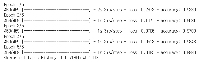

여기서 ,

469 -> 이미지의 갯수를 의미하고 ,
이렇게 나오는 이유는 batch_size를 128로 했기 때문에 60000/128 = 468.5 가 나오기떄문이다.

단순한 Dense 클래스

import tensorflow as tf

class NaiveDense:
    def __init__(self, input_size, output_size, activation):
        self.activation = activation

        w_shape = (input_size, output_size)
        w_initial_value = tf.random.uniform(w_shape, minval=0, maxval=1e-1)
        self.W = tf.Variable(w_initial_value)

        b_shape = (output_size,)
        b_initial_value = tf.zeros(b_shape)
        self.b = tf.Variable(b_initial_value)

    def __call__(self, inputs):
        return self.activation(tf.matmul(inputs, self.W) + self.b)

    @property
    def weights(self):
        return [self.W, self.b]

• init 함수는 입력 크기 input_size, 출력 크기 output_size, 활성화 함수 activation을 인자로 받습니다. 이 클래스의 객체가 만들어질 때 W와 b라는 두 가지 TensorFlow 변수를 생성하게 됩니다. W는 입력과 출력 사이의 가중치(weight)를 나타내며, b는 출력에 더해지는 편향(bias)을 나타냅니다. W는 크기가 (input_size, output_size)이며, 0과 0.1 사이의 균일분포(uniform distribution)로 초기화됩니다. b는 크기가 (output_size,)이며, 0으로 초기화됩니다

• call 함수는 입력 inputs를 받아서 activation 함수를 적용한 결과를 반환합니다. 이 함수는 입력 inputs와 W를 행렬곱하고, b를 더한 후, 그 결과에 activation 함수를 적용한 값을 반환합니다.

• weights 함수는 W와 b 변수를 리스트로 묶어서 반환합니다. 이 함수는 이후 모델 학습에서 변수 업데이트를 위해 사용