Intro
필자들은 Convolution Block Attention Module (CBAM)을 제안한다.
최근의 CNN 성능 향상을 위한 architecture 연구는 크게 3 가지 측면에서 이뤄지고 있다.
- depth
- width
- cardinality
depth와 width의 경우 ResNet, GoogLeNet 등의 논문을 통해 이미 익숙해진 개념이다.
- ResNet에서는 모델의 깊이가 깊어질수록 모델의 성능이 향상됨을 보였다.
- GoogLeNet은 인셉션 모듈에서 모델의 width의 확장을 통해 모델 성능이 향상됐음을 확인했다.
하지만 Cardinality에 대한 내용은 다소 생소할 수 있다.
Cardinality의 개념은 ResNext 논문(Aggregated Residual Transformations for Deep Neural Networks)에서 제안한 개념이다.
Cardinality
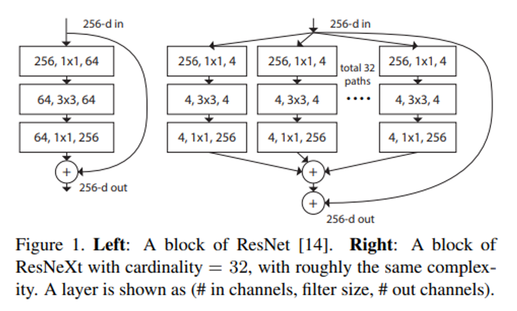
Aggregated Residual Transformations for Deep Neural Networks
ResNeXt is a simple, highly modularized network architecture for image classification. Our network is constructed by repeating a building block that aggregates a set of transformations with the same topology. Our simple design results in a homogeneous, multi-branch architecture that has only a few hyper-parameters to set. This strategy exposes a new dimension, which we call “cardinality” (the size of the set of transformations), as an essential factor in addition to the dimensions of depth and width. [1]
위의 세 가지 트렌드가 언급되었지만 이번 논문에서 집중하는 architecture는 attention이다.
저자가 말하는 Attention의 장점은 다음과 같다.
- 어디에 Focus를 하는지 정보를 제공해준다.
- Representation power를 증가시켜 준다.
저자는 단순히 Attention 알고리즘을 적용하는 것에서 그치는 것이 아니라 2차원으로 데이터를 나눠서 Attention mechanism을 적용하는 것을 제안한다.
- Channel
- Spatial
이것에 대한 더 자세한 설명은 이후 부분에서 보자.
Related Work
Network engineering
모델의 디자인은 성능을 결정하는 매우 중요한 요소 중 하나이다. Intro에서도 설명했듯 최근의 연구는 depth, width, cardinality를 중점적으로 봤다면 이번 논문에서는 Attention mechanism에 중심을 두겠다고 한다.
(해당 논문이 작성된 시가와 현재 차이가 있기 때문에 감안하고 이해해야할듯 하다.)
Attention mechanism
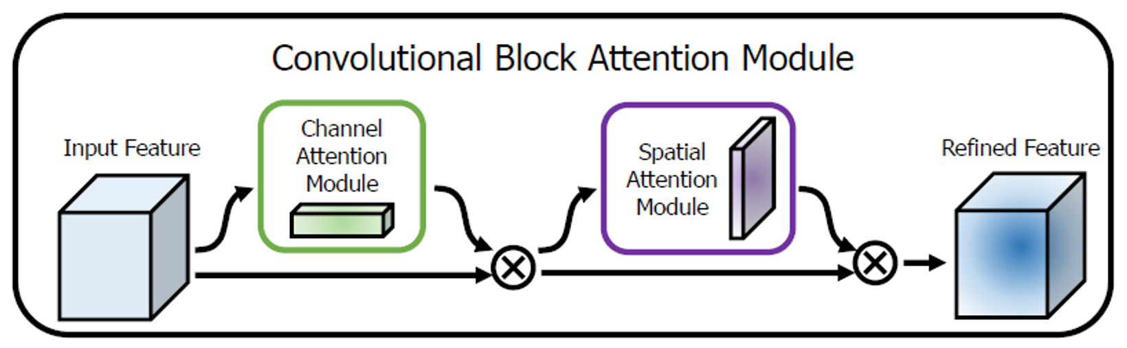
CNN에 attention mechanism을 적용하려는 시도는 많았다. 기존의 방법들과 다른 점은 저자는 3D feature map에 그대로 attention을 적용하는 것이 아니라 3D feature map을 두 가지 축으로 분해를 해서 2번의 attention 계산 과정을 거친다는 점이다.
이번 논문의 핵심이 되는 부분으로 좀 더 자세히 살펴보면
channel에 대해서 attention score를 구한 후 feature map에 곱한 후 spatial (height x width)에 대해서 attention score를 구하는 두 작업으로 나눠서 진행한다.
CBAM
모델 중간의 featurem map이 다음과 같이 주어질 때
CBAM은 순차적으로
1D channel attention map :
2D spatial attention map :
를 추론한다. (아래의 그림 참고.)
위의 과정을 요약하면 다음과 같다. ( : element-wise multiplication)
논문에서는 순차적으로 attention을 배치하는 것이 병렬적으로 배치하는 것보다 효과적임을 보였다.
2단계 attention map 추론 과정
Channel attention module
Channel attention focuses on 'what' is meaningful given an input image
Channel attention을 계산하는 과정은 다음과 같다.
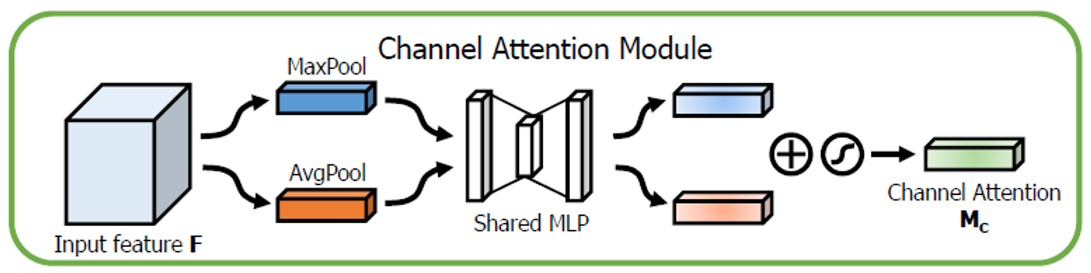
Channel attention module 구하는 방법 도식화
-
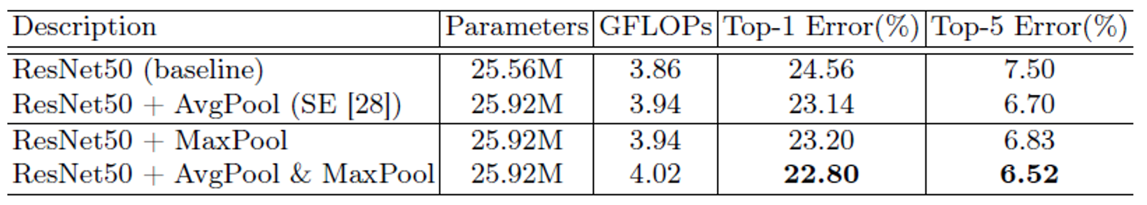
spatial 정보를 Avg pooling과 Max pooling을 사용해 descriptors 와 를 추출한다.
channel attention score를 구하기 위해서 spatial 정보를 압축(통합)할 방법이 필요하다.
기존의 연구들에서는 이 방법으로 Average pooling을 주로 사용했다.
저자들은 여기서 Max pooling 방법도 함께 사용할 것을 제안한다. Max pooling을 통해서 다른 것들과 명확히 구별이 되는 object feature를 잡아낼 수 있다는 게 저자들의 설명이다.
실험적으로도 각각의 pooling 방법을 적용하는 것보다 두 가지를 같이 썼을 때 성능이 더 좋았다고 한다.
-
descriptor 각각을 shared MLP에 넣은 후 결과를 합한다..
parameter를 공유하는 MLP에 각각의 descriptor를 넣는다. MLP는 크기의 hidden layer를 갖는 구조이다. 여기서 r은 reduction ratio를 의미한다.
각각 descriptor에 대한 MLP의 output은 element-wise sum을 통해서 최종 output을 도출한다.
위의 일련의 과정은 다음과 같이 수식화할 수 있다.
Spatial attention module
spatial attention focuses on ‘where’ is an informative part
Spatial attention을 계산하는 과정은 다음과 같다.
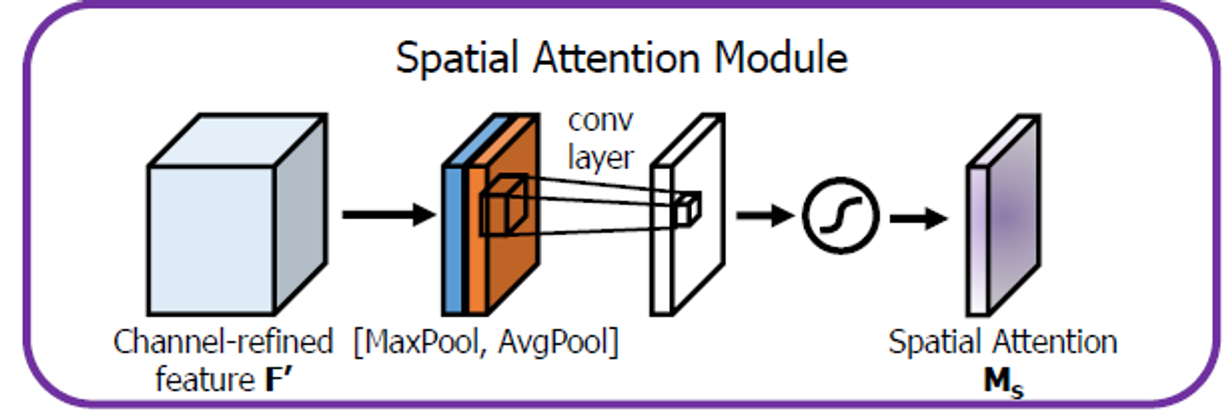
Spatial attention module 구하는 방법 도식화
-
channel 정보를 Avg pooling과 Max pooling을 사용해 descriptors 와 를 추출한다.
방법은 channel attention module에서 방법과 동일하다.
-
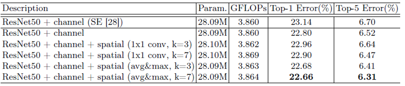
와 를 concat한 후, 7x7 크기를 가진 filter 1개로 attention weight을 계산한다.
그림을 통해서 충분히 이해가 가능할 것이다.
위의 일련의 과정은 다음과 같이 수식화할 수 있다.
Experiments
ablation experiments
모델이나 알고리즘의 특징들을 제거하면서 그게 퍼포먼스에 어떤 영향을 줄지 연구하는 것 [2]
1. channel attention
Max pooling과 Avg pooling의 영향 검증.
2. Spatital attention
Max pooling, Avg pooling 그리고 kernel size의 영향 검증.
3. Arrangement of the channel and spatial attention
각 attention의 순차적, 병렬적 배치 및 순서에 따른 영향 검증.
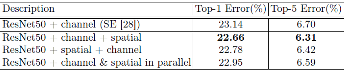
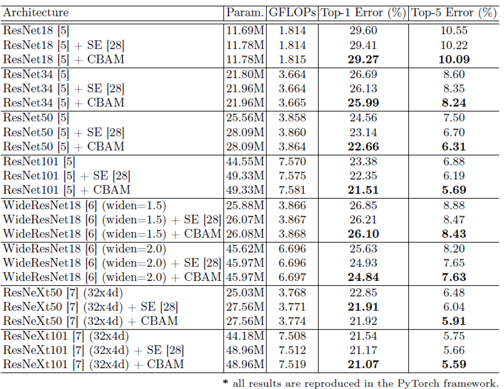
Image Classification on ImageNet - 1K
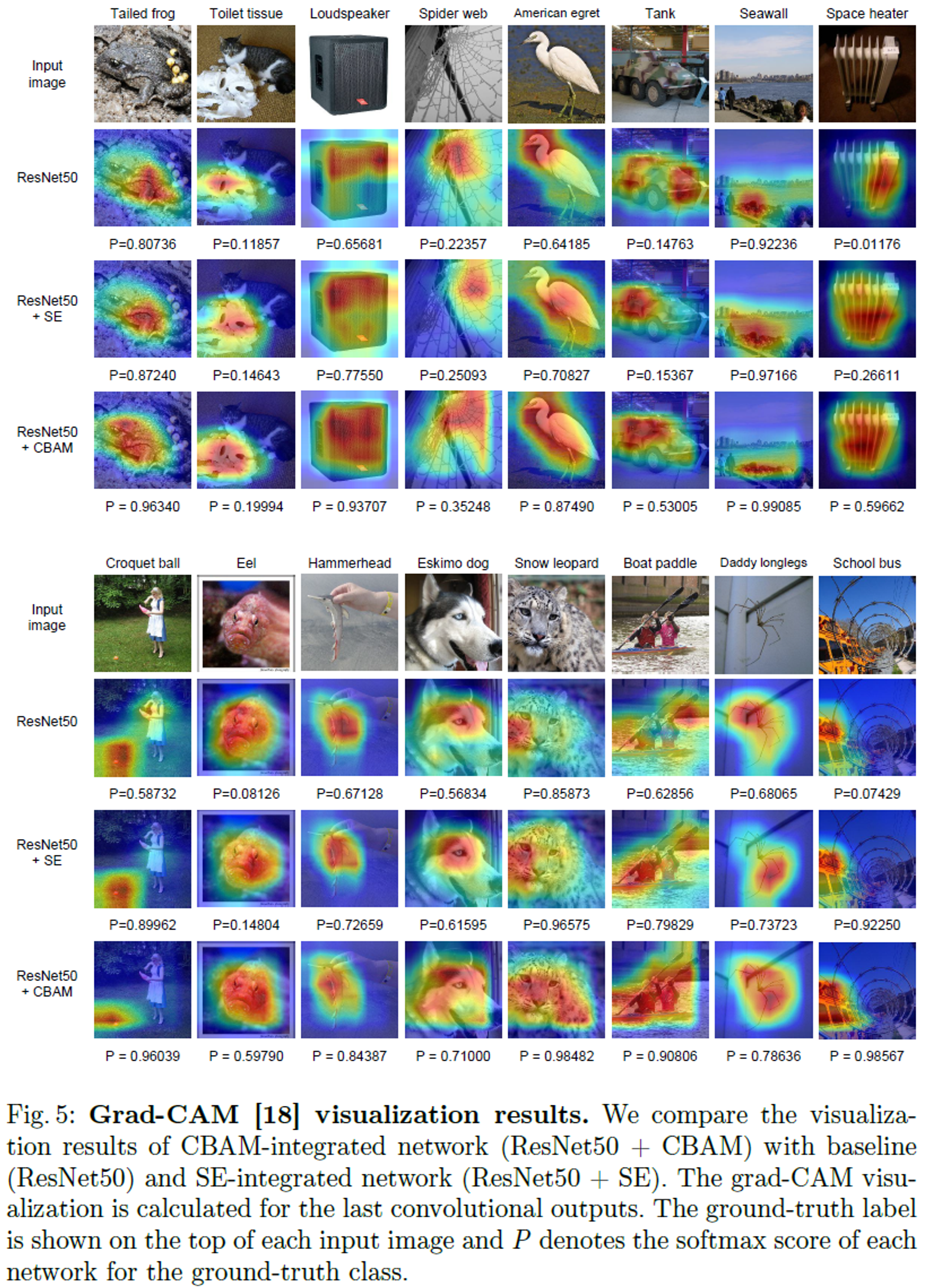
Network Visualization with Grad-CAM
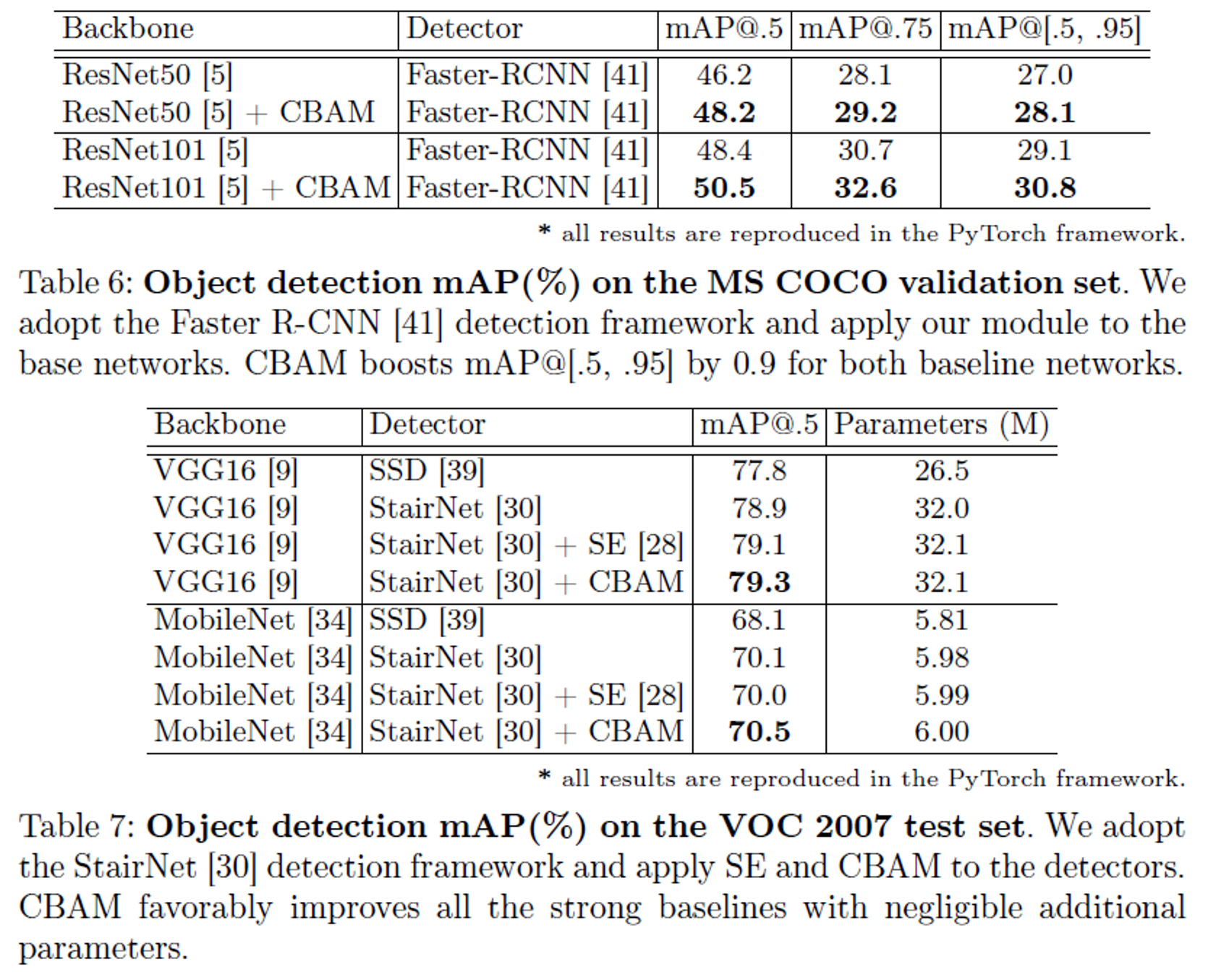
MS COCO & VOC 2007 Object Detection
Reference
[1][https://github.com/facebookresearch/ResNeXt](https://github.com/facebookresearch/ResNeXt)
[2][https://study-grow.tistory.com/37](https://study-grow.tistory.com/37)