
시계열 튜토리얼
jupyter notbook환경에서 하고 싶었지만 Prophet 다운이 모두 잘 되었지만 버전에 오류가 자꾸 생겨 google colabatory환경에서 진행했다.
- 모듈 다운
- window환경
- Visual C++ Build Tool을 먼저 설치해야 한다.
- conda install pandas-datareader
- conda install -c conda-forge fbprophet
1) 사인(sin)함수를 그리는 함수를 만들기
- a = 진폭
- f = 주기
- t0 = 시작 시간
- b = bias:y축 중심
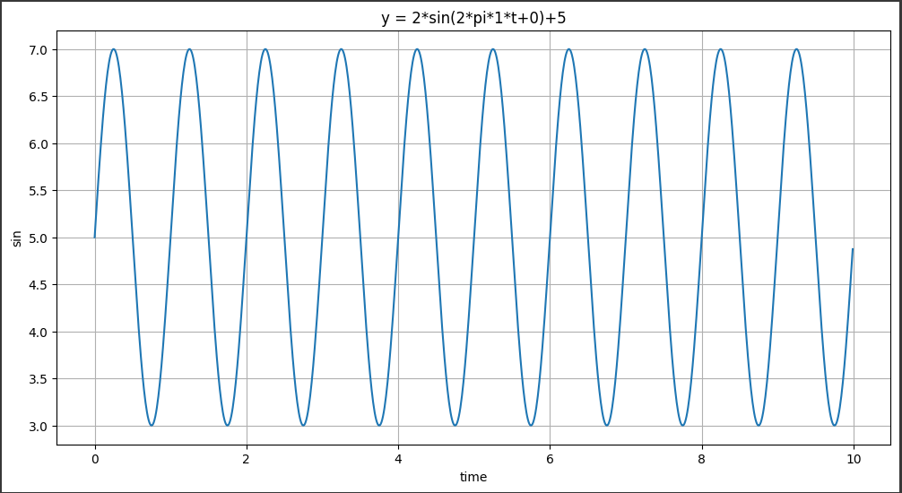
def plotSinWave(amp, freq, endTime, sampleTime, startTime, bias):
    """
    plot sine wave
    y = a sin(2 pi f t + t_0) + b
    """
    time = np.arange(startTime, endTime, sampleTime)
    result = amp * np.sin(2 * np.pi * freq * time + startTime) + bias

#그래프 그리기
    plt.figure(figsize=(12, 6))
    plt.plot(time, result)
    plt.grid(True)
    plt.xlabel("time")
    plt.ylabel("sin")

    plt.title("y = "+str(amp) + "*sin(2*pi*" + str(freq) + "*t+" +
    str(startTime) + ")+" + str(bias))

    plt.show()
- 함수 호출
plotSinWave(2, 1, 10, 0.01, 0, 5)

sin함수 호출 시 매개변수의 값을 모른다면? ( 함수명(**): )
- """ 내용 """ : 해당 함수의 설명 = 내용
- 매개변수의 값을 모르거나 그때그떄 변경해야 한다면 변수마다 기본값을 설정하고 상황에 따라 값을 넣어주면 된다.
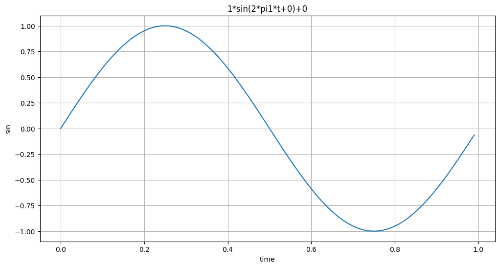
def plotSinWave(**kwargs):
    """
    plot sine wave
    y = a sin(2 pi f t + t_0) + b
    """

#매개변수 기본값 설정
    endTime = kwargs.get("endTime", 1)
    sampleTime = kwargs.get("sampleTime", 0.01)
    amp = kwargs.get("amp", 1)
    freq = kwargs.get("freq", 1)
    startTime = kwargs.get("startTime", 0)
    bias = kwargs.get("bias", 0)
    figsize = kwargs.get("figsize", (12, 6))

    time = np.arange(startTime, endTime, sampleTime)
    result = amp * np.sin(2 * np.pi * freq * time + startTime) + bias

#그래프 그리기
    plt.figure(figsize=(12, 6))
    plt.plot(time, result)
    plt.grid(True)
    plt.xlabel("time")
    plt.ylabel("sin")

    plt.title(str(amp) + "*sin(2*pi" + str(freq) +
    "*t+" + str(startTime) + ")+" + str(bias))

    plt.show()
- 함수 호출1
plotSinWave() : 설정해 놓은 기본 값들이 매개변수
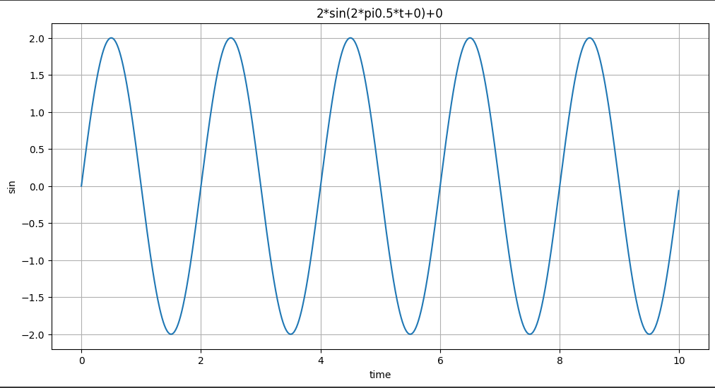
- 함수 호출2
plotSinWave(amp=2, freq=0.5, endTime=10)
2) 내가 만든 함수 Import해서 사용하기
- 위에서 만든 sin함수 그리는 함수(plotSinWave(**kwargs)) .py파일로 저장
- pycharm에서 실제 py파일을 만들어 함수 작성 후 저장
- %%writefile ./모듈명.py 사용
- 2번 방법으로 해보자
%%writefile ./drawSinWave.py

import numpy as np
import matplotlib.pyplot as plt

def plotSinWave(**kwargs):
    """
    plot sine wave
    y = a sin(2 pi f t + t_0) + b
    """
    endTime = kwargs.get("endTime", 1)
    sampleTime = kwargs.get("sampleTime", 0.01)
    amp = kwargs.get("amp", 1)
    freq = kwargs.get("freq", 1)
    startTime = kwargs.get("startTime", 0)
    bias = kwargs.get("bias", 0)
    figsize = kwargs.get("figsize", (12, 6))

    time = np.arange(startTime, endTime, sampleTime)
    result = amp * np.sin(2 * np.pi * freq * time + startTime) + bias

    plt.figure(figsize=(12, 6))
    plt.plot(time, result)
    plt.grid(True)
    plt.xlabel("time")
    plt.ylabel("sin")
    plt.title(str(amp) + "*sin(2*pi" + str(freq) + "*t+" +
    str(startTime) + ")+" + str(bias))
    plt.show()

if __name__ == "__main__":
    print("hello world~!!")
    print("this is test graph!!")
    plotSinWave(amp=1, endTime=2)
위에서 만든 함수의 내용과 다른점이 있다.
if문이 추가 되었다.
무엇인지 알아보자if __name__ == "__main__": print("hello world~!!") print("this is test graph!!") plotSinWave(amp=1, endTime=2)말로 풀어보면
만약 만든 .py 파일이 파이썬에서 직접 실행파일로 사용 된다면 if문을 실행해라
라는 코드이다.반대로 .py파일이 모듈로 import가 된다면 if문은 실행되지 않고 함수의 기능만 실행 될 것이고 실행된다.
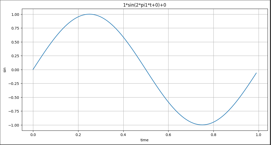
- 실제로 만든 모듈을 사용해 보자
import drawSinWave as dS
dS.plotSinWave()
dS.plotSinWave(freq=5)

이제 본격적으로 fbprophet을 사용해 보자
모듈 import
import pandas as pd
import numpy as np
import matplotlib.pyplot as plt
%matplotlib inline
- 그래프로 표현 할 데이터 프레임 만들기
- linesapce(시작, 끝, 시작~끝등분 수) :
time = np.linspace(0, 1, 365*2)
result = np.sin(2*np.pi*12*time)
ds = pd.date_range("2018-01-01", periods=365*2, freq="D")
df = pd.DataFrame({"ds": ds, "y": result})
df.head()

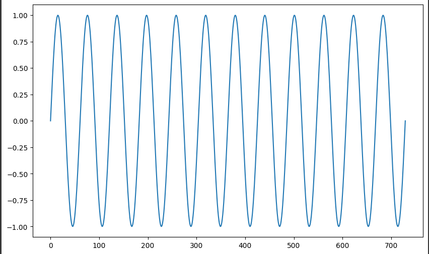
- 만든 데이터 프레임으로 그래프 그리기
- 가장 뒤 ; 은 시각화된 그래프에 나오는 다른 글들을 지워준다.
df["y"].plot(figsize=(10, 6));
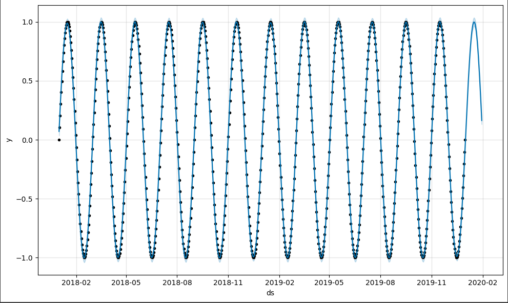
- Prophet 함수
- 현재 데이터의 경향성으로 추후 30일 미래 데이터를 예측
from prophet import Prophet

m = Prophet(yearly_seasonality=True, daily_seasonality=True)
m.fit(df);
future = m.make_future_dataframe(periods=30)
forecast = m.predict(future)
m.plot(forecast);
- 점 찍힌 부분이 분석한 데이터들이고 뒤의 그냥 선이 예측한 데이터이다.
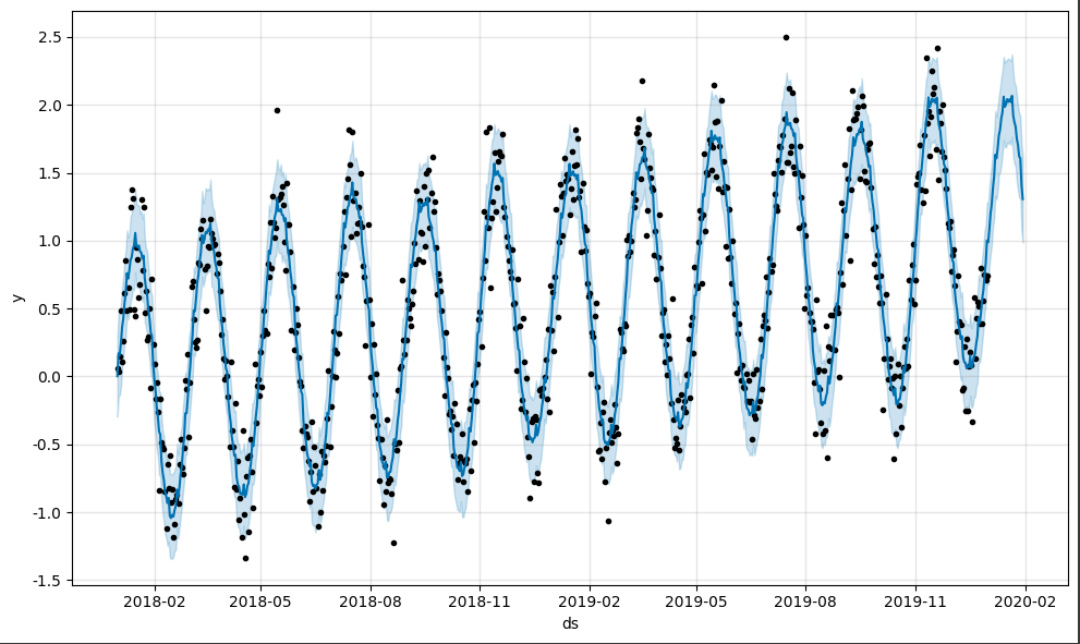
좀 더 어려운 예측을 해보자
- 난수로 노이즈식의 데이터 만들어 prophet으로 예측시켜 보자
- 함수 만들기
time = np.linspace(0, 1, 365*2)
result = np.sin(2*np.pi*12*time) + time + np.random.randn(365*2)/4

ds = pd.date_range("2018-01-01", periods=365*2, freq="D")
df = pd.DataFrame({"ds": ds, "y": result})

df["y"].plot(figsize=(10, 6));
- prophet으로 예측 해보기
m = Prophet(yearly_seasonality=True, daily_seasonality=True)
m.fit(df)
future = m.make_future_dataframe(periods=30)
forecast = m.predict(future)
m.plot(forecast);

처음으로 코딩을 배우면서 신기하다라는 생각을 했다.
미래를 예측한다고?
정말 예측한 결과가 맞을까?
데이터가 많을 수록 예측 결과가 맞을 확률이 높아지나?
로또번호 예측이 가능 할까?????
3) 블로그 방문자수 예측
강사님이 따로 블로그 운영을 하신다고 한다.
멋지시다.
강사님 블로그의 방문자수를 예측해보자
데이터(.csv)파일은 강의에서 제공해 주셨다.
- 모듈 import
import pandas as pd
import pandas_datareader as web
import numpy as np
import matplotlib.pyplot as plt

from prophet import Prophet
from datetime import datetime

%matplotlib inline
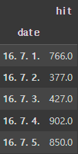
- csv파일 불러오기
pinkwink_web = pd.read_csv(
    "/content/drive/MyDrive/Colab Notebooks
    /05_PinkWink_Web_Traffic.csv",

    encoding="utf-8",
    thousands=",",
    names=["date", "hit"],
    index_col=0
)

pinkwink_web = pinkwink_web[pinkwink_web["hit"].notnull()]
pinkwink_web.head()
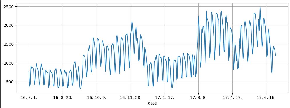
- 전체 데이터 그려보기
pinkwink_web["hit"].plot(figsize=(12, 4), grid=True);
- trend 분석을 시각화하기 위한 x축 값 만들기
time = np.arange(0, len(pinkwink_web))
traffic = pinkwink_web["hit"].values
fx = np.linspace(0, time[-1], 1000)
- 에러 계산할 함수 만들기
- 예측값에서 참값을 뺀것이 에러
- 트랜드를 만들어서 트랜드가 얼마나 원데이터를 반영 했는지 확인하기 위해
- f : 함수, x : 받아들이는 값 , y : 참값
- rnse 라고도 부른다.
def error(f, x, y):
    return np.sqrt(np.mean((f(x) - y) ** 2))
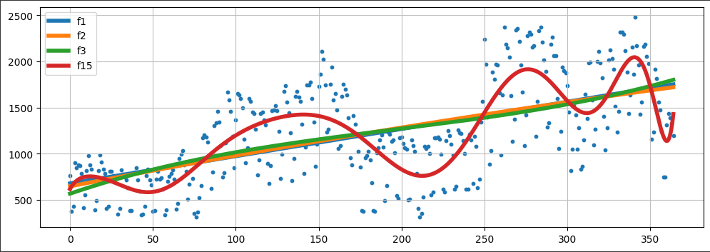
- 상관계수 구해서 경향선 만들기
#1차원
f1p = np.polyfit(time, traffic, 1)
f1 = np.poly1d(f1p)

2차원
f2p = np.polyfit(time, traffic, 2)
f2 = np.poly1d(f2p)

3차원
f3p = np.polyfit(time, traffic, 3)
f3 = np.poly1d(f3p)

15차원
f15p = np.polyfit(time, traffic, 15)
f15 = np.poly1d(f15p)
- 에러 구하기
print(error(f1, time, traffic))
print(error(f2, time, traffic))
print(error(f3, time, traffic))
print(error(f15, time, traffic))
430.8597308110963 430.6284101894695 429.53280466762925 330.4777305877038
- 구한 트랜드를 그려보자
plt.figure(figsize=(12, 4))
plt.scatter(time, traffic, s=10)
plt.plot(fx, f1(fx), lw=4, label='f1')
plt.plot(fx, f2(fx), lw=4, label='f2')
plt.plot(fx, f3(fx), lw=4, label='f3')
plt.plot(fx, f15(fx), lw=4, label='f15')

plt.grid(True, linestyle="-", color="0.75")
plt.legend(loc=2)
plt.show()
여태까지는 트랜드를 구해보았다.
이제는 실제 예측을 해보자.
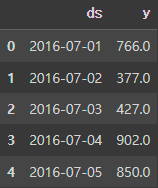
- prophet에 사용할 데이터 프레임 만들기
df = pd.DataFrame({"ds": pinkwink_web.index, "y": pinkwink_web["hit"]})
df.reset_index(inplace=True)
df["ds"] = pd.to_datetime(df["ds"], format="%y. %m. %d.")
del df["date"]
df.head()
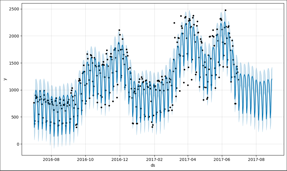
- 예측 값
m = Prophet(yearly_seasonality=True, daily_seasonality=True)
m.fit(df);
# 60일에 해당하는 데이터 예측
future = m.make_future_dataframe(periods=60)
future.tail()
- 예측 결과는 상/하한의 범위를 포함해서 얻어진다.
forecast = m.predict(future)
forecast[["ds", "yhat", "yhat_lower", "yhat_upper"]].tail()
- 예측 값 그려보기
m.plot(forecast);


취업공부