A Diffusion Model from Scratch in Pytorch

해당 포스트에서는 자동차 이미지로 간단한 diffusion 모델을 생성하는 방법을 포스팅 할 것이다. 상세 소스코드와 설명은 아래 링크를 참조하면 될 것이다.

[Sources]
Github : https://github.com/lucidrains/denoising-diffusion-pytorch
Colab notebook : https://colab.research.google.com/drive/1sjy9odlSSy0RBVgMTgP7s99NXsqglsUL?usp=sharing#scrollTo=HhIgGq3za0yh
YouTube : https://www.youtube.com/watch?v=a4Yfz2FxXiY

Investigating the dataset

데이터 세트로 우리는 약 8,000개의 이미지로 구성된 Standord Cars 데이터 세트를 사용합니다.

import torch
import torchvision
import matplotlib.pyplot as plt

def show_images(datset, num_samples=20, cols=4):
    """ Plots some samples from the dataset """
    plt.figure(figsize=(15,15)) 
    for i, img in enumerate(data):
        if i == num_samples:
            break
        plt.subplot(int(num_samples/cols) + 1, cols, i + 1)
        plt.imshow(img[0])

data = torchvision.datasets.StanfordCars(root=".", download=True)
show_images(data)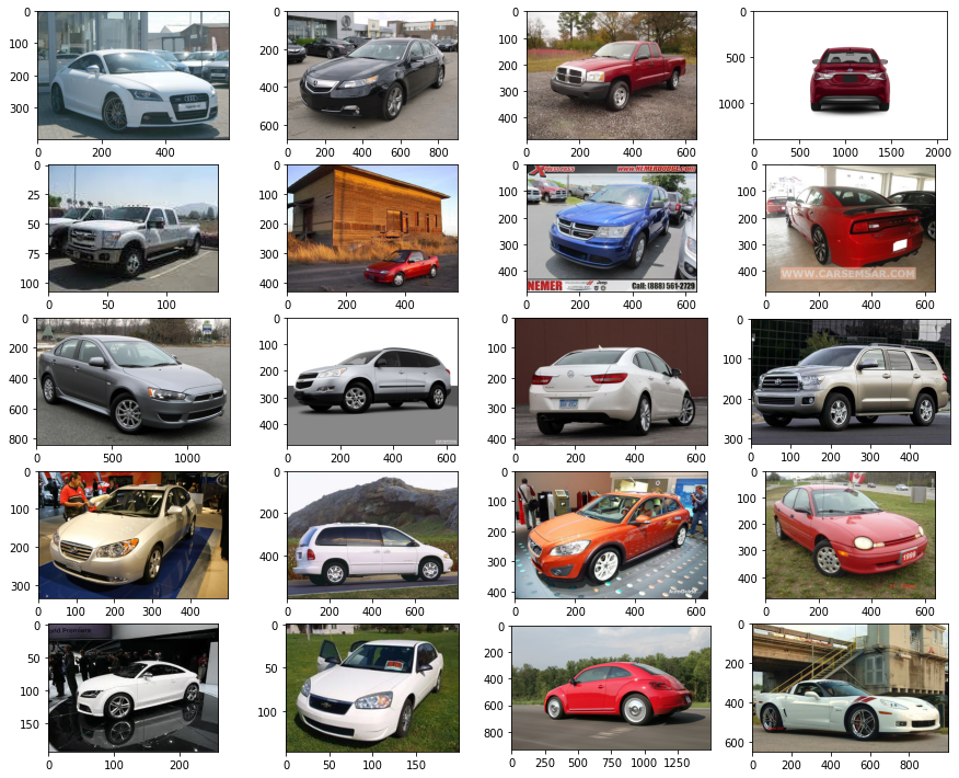

추후 상기 이미지에 transform을 적용한 후 텐서로 변환하여 학습에 사용할 예정입니다.

Building the Diffusion Model

Step 1: The forward process = Noise scheduler

Diffusion 모델이므로 forward로 진행하면서 점점 더 노이즈가 포함된 이미지를 생성할 것입니다. 상기 논문에서는 closed form을 사용하여 각 timestep에 대한 이미지를 개별적으로 계산할 수 있습니다.

[주요 사항]

• noise-levels/variance을 미리 계산할 수 있습니다
• 다양한 유형의 분산 스케줄이 있습니다
• 각 타임스텝 이미지를 독립적으로 샘플링할 수 있습니다(가우시안의 합도 가우시안)
• forward 단계에서는 모델이 필요하지 않습니다

import torch.nn.functional as F

def linear_beta_schedule(timesteps, start=0.0001, end=0.02):
    return torch.linspace(start, end, timesteps)

def get_index_from_list(vals, t, x_shape):
    """ 
    Returns a specific index t of a passed list of values vals
    while considering the batch dimension.
    """
    batch_size = t.shape[0]
    out = vals.gather(-1, t.cpu())
    return out.reshape(batch_size, *((1,) * (len(x_shape) - 1))).to(t.device)

def forward_diffusion_sample(x_0, t, device="cpu"):
    """ 
    Takes an image and a timestep as input and 
    returns the noisy version of it
    """
    noise = torch.randn_like(x_0)
    sqrt_alphas_cumprod_t = get_index_from_list(sqrt_alphas_cumprod, t, x_0.shape)
    sqrt_one_minus_alphas_cumprod_t = get_index_from_list(
        sqrt_one_minus_alphas_cumprod, t, x_0.shape
    )
    # mean + variance
    return sqrt_alphas_cumprod_t.to(device) * x_0.to(device) \
    + sqrt_one_minus_alphas_cumprod_t.to(device) * noise.to(device), noise.to(device)


# Define beta schedule
T = 300
betas = linear_beta_schedule(timesteps=T)

# Pre-calculate different terms for closed form
alphas = 1. - betas
alphas_cumprod = torch.cumprod(alphas, axis=0)
alphas_cumprod_prev = F.pad(alphas_cumprod[:-1], (1, 0), value=1.0)
sqrt_recip_alphas = torch.sqrt(1.0 / alphas)
sqrt_alphas_cumprod = torch.sqrt(alphas_cumprod)
sqrt_one_minus_alphas_cumprod = torch.sqrt(1. - alphas_cumprod)
posterior_variance = betas * (1. - alphas_cumprod_prev) / (1. - alphas_cumprod)

현재 데이터셋에 적용을 하면 다음과 같습니다.

from torchvision import transforms 
from torch.utils.data import DataLoader
import numpy as np

IMG_SIZE = 64
BATCH_SIZE = 128

def load_transformed_dataset():
    data_transforms = [
        transforms.Resize((IMG_SIZE, IMG_SIZE)),
        transforms.RandomHorizontalFlip(),
        transforms.ToTensor(), # Scales data into [0,1] 
        transforms.Lambda(lambda t: (t * 2) - 1) # Scale between [-1, 1] 
    ]
    data_transform = transforms.Compose(data_transforms)

    train = torchvision.datasets.StanfordCars(root=".", download=True, 
                                         transform=data_transform)

    test = torchvision.datasets.StanfordCars(root=".", download=True, 
                                         transform=data_transform, split='test')
    return torch.utils.data.ConcatDataset([train, test])
def show_tensor_image(image):
    reverse_transforms = transforms.Compose([
        transforms.Lambda(lambda t: (t + 1) / 2),
        transforms.Lambda(lambda t: t.permute(1, 2, 0)), # CHW to HWC
        transforms.Lambda(lambda t: t * 255.),
        transforms.Lambda(lambda t: t.numpy().astype(np.uint8)),
        transforms.ToPILImage(),
    ])

    # Take first image of batch
    if len(image.shape) == 4:
        image = image[0, :, :, :] 
    plt.imshow(reverse_transforms(image))

data = load_transformed_dataset()
dataloader = DataLoader(data, batch_size=BATCH_SIZE, shuffle=True, drop_last=True)

# Simulate forward diffusion
image = next(iter(dataloader))[0]

plt.figure(figsize=(15,15))
plt.axis('off')
num_images = 10
stepsize = int(T/num_images)

for idx in range(0, T, stepsize):
    t = torch.Tensor([idx]).type(torch.int64)
    plt.subplot(1, num_images+1, int(idx/stepsize) + 1)
    img, noise = forward_diffusion_sample(image, t)
    show_tensor_image(img)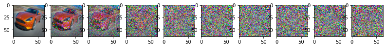

Step 2: The backward process = U-Net

[주요 사항]

• 이미지의 노이즈를 예측하기 위해 간단한 형태의 UNet을 사용합니다
• 입력은 노이즈 이미지이며, 이미지의 노이즈를 출력합니다
• 매개변수가 시간에 따라 공유되기 때문에 네트워크에 어느 시간 단계에 있는지 알려야 합니다
• Timesstep은 트랜스포머 Sinosoidal Embedding에 의해 인코딩됩니다
• 분산이 고정되어 있으므로 단일 값(평균)을 하나 출력합니다

from torch import nn
import math


class Block(nn.Module):
    def __init__(self, in_ch, out_ch, time_emb_dim, up=False):
        super().__init__()
        self.time_mlp =  nn.Linear(time_emb_dim, out_ch)
        if up:
            self.conv1 = nn.Conv2d(2*in_ch, out_ch, 3, padding=1)
            self.transform = nn.ConvTranspose2d(out_ch, out_ch, 4, 2, 1)
        else:
            self.conv1 = nn.Conv2d(in_ch, out_ch, 3, padding=1)
            self.transform = nn.Conv2d(out_ch, out_ch, 4, 2, 1)
        self.conv2 = nn.Conv2d(out_ch, out_ch, 3, padding=1)
        self.bnorm1 = nn.BatchNorm2d(out_ch)
        self.bnorm2 = nn.BatchNorm2d(out_ch)
        self.relu  = nn.ReLU()
        
    def forward(self, x, t, ):
        # First Conv
        h = self.bnorm1(self.relu(self.conv1(x)))
        # Time embedding
        time_emb = self.relu(self.time_mlp(t))
        # Extend last 2 dimensions
        time_emb = time_emb[(..., ) + (None, ) * 2]
        # Add time channel
        h = h + time_emb
        # Second Conv
        h = self.bnorm2(self.relu(self.conv2(h)))
        # Down or Upsample
        return self.transform(h)


class SinusoidalPositionEmbeddings(nn.Module):
    def __init__(self, dim):
        super().__init__()
        self.dim = dim

    def forward(self, time):
        device = time.device
        half_dim = self.dim // 2
        embeddings = math.log(10000) / (half_dim - 1)
        embeddings = torch.exp(torch.arange(half_dim, device=device) * -embeddings)
        embeddings = time[:, None] * embeddings[None, :]
        embeddings = torch.cat((embeddings.sin(), embeddings.cos()), dim=-1)
        # TODO: Double check the ordering here
        return embeddings


class SimpleUnet(nn.Module):
    """
    A simplified variant of the Unet architecture.
    """
    def __init__(self):
        super().__init__()
        image_channels = 3
        down_channels = (64, 128, 256, 512, 1024)
        up_channels = (1024, 512, 256, 128, 64)
        out_dim = 3 
        time_emb_dim = 32

        # Time embedding
        self.time_mlp = nn.Sequential(
                SinusoidalPositionEmbeddings(time_emb_dim),
                nn.Linear(time_emb_dim, time_emb_dim),
                nn.ReLU()
            )
        
        # Initial projection
        self.conv0 = nn.Conv2d(image_channels, down_channels[0], 3, padding=1)

        # Downsample
        self.downs = nn.ModuleList([Block(down_channels[i], down_channels[i+1], \
                                    time_emb_dim) \
                    for i in range(len(down_channels)-1)])
        # Upsample
        self.ups = nn.ModuleList([Block(up_channels[i], up_channels[i+1], \
                                        time_emb_dim, up=True) \
                    for i in range(len(up_channels)-1)])
        
        # Edit: Corrected a bug found by Jakub C (see YouTube comment)
        self.output = nn.Conv2d(up_channels[-1], out_dim, 1)

    def forward(self, x, timestep):
        # Embedd time
        t = self.time_mlp(timestep)
        # Initial conv
        x = self.conv0(x)
        # Unet
        residual_inputs = []
        for down in self.downs:
            x = down(x, t)
            residual_inputs.append(x)
        for up in self.ups:
            residual_x = residual_inputs.pop()
            # Add residual x as additional channels
            x = torch.cat((x, residual_x), dim=1)           
            x = up(x, t)
        return self.output(x)

model = SimpleUnet()
print("Num params: ", sum(p.numel() for p in model.parameters()))
model

Step 3: The loss

def get_loss(model, x_0, t):
    x_noisy, noise = forward_diffusion_sample(x_0, t, device)
    noise_pred = model(x_noisy, t)
    return F.l1_loss(noise, noise_pred)

Training

from torch.optim import Adam

device = "cuda" if torch.cuda.is_available() else "cpu"
model.to(device)
optimizer = Adam(model.parameters(), lr=0.001)
epochs = 100 # Try more!

for epoch in range(epochs):
    for step, batch in enumerate(dataloader):
      optimizer.zero_grad()

      t = torch.randint(0, T, (BATCH_SIZE,), device=device).long()
      loss = get_loss(model, batch[0], t)
      loss.backward()
      optimizer.step()

      if epoch % 5 == 0 and step == 0:
        print(f"Epoch {epoch} | step {step:03d} Loss: {loss.item()} ")
        sample_plot_image()